Formula for Total in Excel: How to Choose the Right Option

Struggling to figure out the right formula for total in Excel? You’re not alone. Excel has several different ways to total numbers, and knowing when to use each one can make the difference between fumbling through a spreadsheet and showing confidence in front of your boss — or even in a job interview.

This guide explains the different options for totalling in Excel and, more importantly, when to use each one. By the end, you’ll know how to save time, avoid mistakes, and prove you know your stuff.

Excel Practice Files

Quick Excel Totals Using the Status Bar

Sometimes you don’t need to write a formula at all. If you want to check a total quickly — for example, adding up the sales for the week before a meeting, or double-checking an invoice — Excel’s status bar can give you the answer instantly. This is great when you don’t want to clutter your sheet with extra formulas.

Steps:

1. Highlight the range of numbers you want to total.
2. Look at the status bar at the bottom of Excel.
3. The total (Sum) will appear instantly.

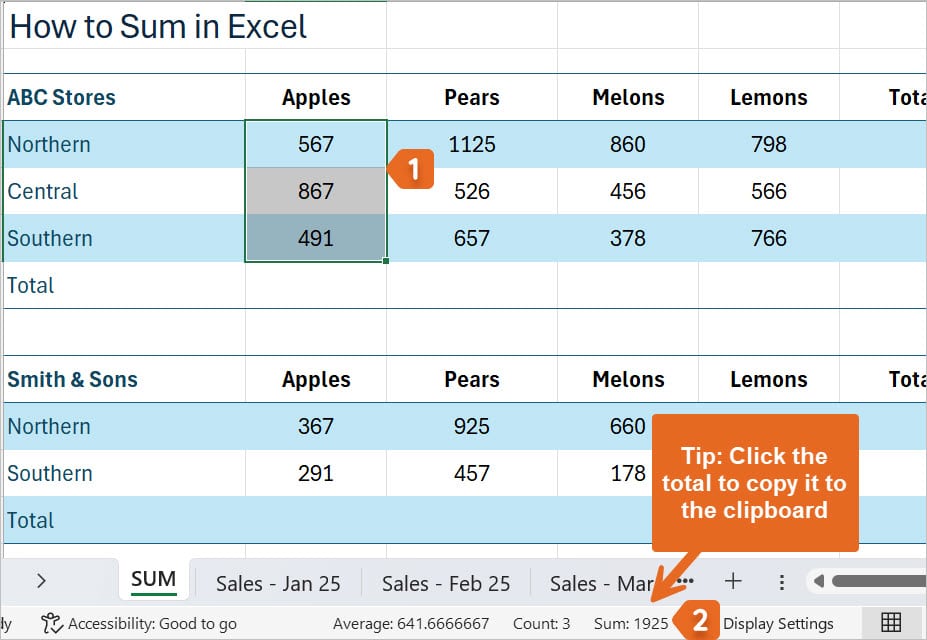
Tip: In Microsoft 365, click the Sum result to copy the result to the clipboard, so you can paste it elsewhere. You can do the same for the Average and Count results.

Total with SUM formula in Excel

The SUM function is the go-to formula for totals in Excel. Think of it as your digital calculator. You use it whenever you need to add up a list of numbers in a clean, reliable way.

Steps to insert a SUM formula:

1. Click the cell where you want the total to appear.
2. Type =SUM(
3. Select the range of numbers you want to add (e.g., B4:B6).
4. Close the bracket ) and press Enter.

Tip: Use the keyboard shortcut Alt + = to quickly insert the SUM formula below or beside your data. First, select the cell that will hold the total. Press Alt + =. Select the range to be totalled and then press Enter. For a full list of Time‑saving Excel shortcuts, check my Best Keyboard Shortcuts for Excel.

SUM Formula Error in Excel – Circular Reference

Even though SUM is simple, it’s easy to make a mistake if you’re in a rush. The most common error happens when you accidentally include the total cell itself inside the formula. This creates a “circular reference” — Excel ends up trying to include its own answer in the calculation.

❌ Wrong: =SUM(B4:B7)
✔️ Correct: =SUM(B4:B6)

To fix this problem, make sure you don’t include the total cell itself (e.g., B7) in your formula range. If you do, Excel will attempt to add the answer to itself, resulting in a circular reference error.

Formula to Total Rows and Columns at the Same Time

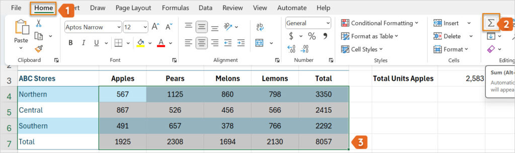
If you’re dealing with a large block of numbers — for example, a monthly sales report where each row is a region and each column is a product — you don’t want to waste time writing a formula for every row and every column. Excel has a shortcut that totals everything at once.

Steps:

1. Select the whole block of numbers plus one blank row and one blank column.

2. From the Home tab, click the Sum button, or press Alt + = on your keyboard.
3. Excel will insert totals for every row and column automatically.

Formula to SUM Across Multiple Sheets in Excel

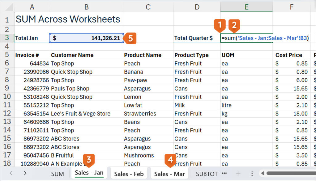
Sometimes your data is spread across different sheets — maybe one sheet for January, one for February, and one for March. Instead of writing three separate SUM formulas, you can use a 3D SUM to pull everything together.

Essential Checks Before Using 3D SUM

• Check that the cell or range you want to total is in the same position on every worksheet you’re including in your 3D SUM formula. For example, if you’re totalling cell B3, make sure B3 contains the value you want to sum on each sheet.
• All the worksheets you want to include must be adjacent in your workbook. The formula references a continuous block of sheets, from the first to the last tab you select. You can’t include non-adjacent (separated) sheets in a single 3D SUM formula.

Steps:

1. Click in the cell where you want the total to appear.
2. Type =SUM(
3. Click the first sheet tab (e.g., Sales – Jan).
4. Hold Shift and click the last sheet tab (e.g., Sales – Mar).
5. Select the cell you want to total from each of the selected sheets (e.g., B3).
6. Press Enter.

Formula to Sum Only Filtered Data in Excel

Creating a formula to total filtered data can be tricky. This is where the SUBTOTAL function comes in.

Both SUM and SUBTOTAL add numbers, but the key difference lies in how they handle hidden rows and filtered data.

If you use SUM, Excel adds everything, even the rows you’ve hidden. But SUBTOTAL only totals the rows you can currently see — perfect when you want to drill down into filtered reports.

Steps to use SUBTOTAL:

1. Filter your data (e.g., using column filters).
2. Click the cell where you want the total.
3. Type =SUBTOTAL(9, then type or select your range (e.g., F4:F24).
4. Press Enter.

For more information on using SUBTOTAL with Filter, check out my blog ‘How to Sum only visible cells in Excel when using Filter’.

Formula to Total Only What You Need in Excel (SUMIF)

The SUMIF function enables you to calculate the total of numbers that meet a specific condition. Think of it as telling Excel: “Only total these if they match this rule.” In the example below, we want to calculate the total sales to the customer “Top Shop”.

Steps:

1. Click the cell where you want the total.
2. Type =SUMIF(
3. Select the criteria range. This is the group of cells that contains the values you want Excel to check or match when deciding which numbers to total (for example, selecting A7:A23 asks Excel to look down the Customer Name column).
4. Type a comma, then enter your condition (the value you want to total). You can type a specific value, or you can enter the cell reference that contains the value you want to match (e.g., A4). If entering text, don’t forget to use double-quote marks around the text, e.g. “Top Shop”.
5. Type a comma, then select the sum range, the group of cells that contains the numbers you want to add up if they meet your condition (for example, E7:E23).
6. Close the bracket and press Enter.

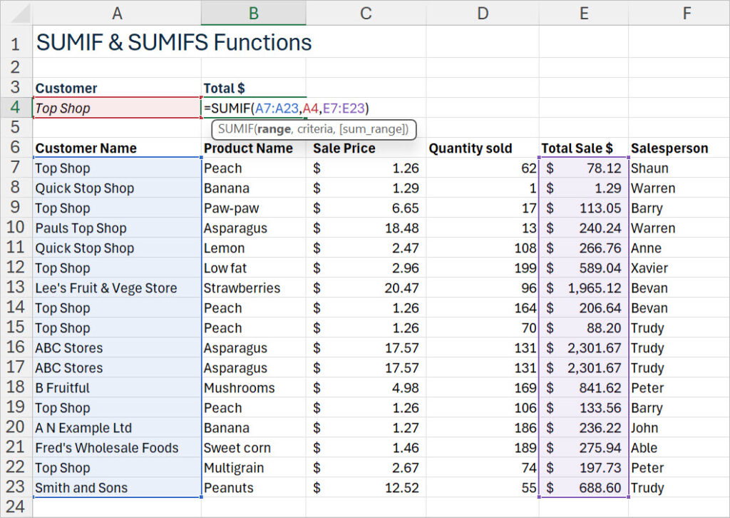
Excel will only total the rows where the value in your criteria range matches the specified value, e.g., “Top Shop”.

Did you know you can use the SUMIF function to create a formula to total ranges that include errors? Check out my blog post ‘How do I sum a range of cells that include #N/A or #DIV/0! Errors?’

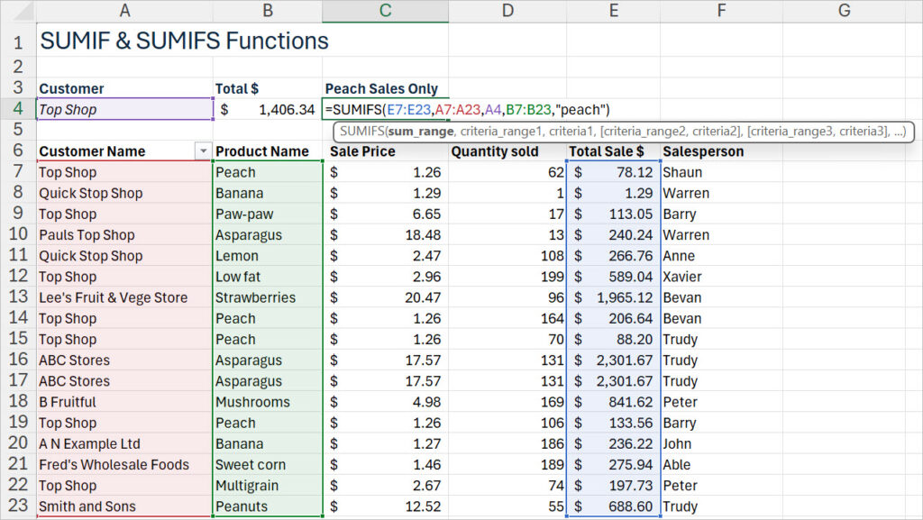
SUMIF with Multiple Criteria (SUMIFS)

SUMIFS builds on SUMIF, allowing you to apply multiple conditions simultaneously.

Steps:

1. Click the cell where you want the result to appear. In this example, the cell is C4.
2. Type =SUMIFS( to start your formula.
3. Select the sum range. This is the group of cells containing the numbers you want to add up if they meet all your conditions. Example: E7:E23 (the “Total Sale $” column).
4. Type a comma, then select the first criteria range. This is the range where Excel will look for your first condition. Example: A7:A23 (the “Customer Name” column).
5. Type a comma, then enter your first condition. You can type a value in double quotes (e.g., “Top Shop”), or use a cell reference (e.g., A4). In the example, A4 contains “Top Shop”.
6. Type a comma, then select the second criteria range. This is the next group of cells where Excel will check your second condition. Example: B7:B23 (the “Product Name” column).
7. Type a comma, then enter your second condition. Again, use double quotes for a specific value (e.g., “peach”), or a cell reference. In the example, “peach” is typed directly.
8. Close the bracket and press Enter.

Excel will add up all the values in the “Total Sale $” column (E7:E23) where the “Customer Name” is “Top Shop” (from A7:A23) and the “Product Name” is “peach” (from B7:B23).

Tip: You can add more criteria by repeating the pattern: comma, criteria range, comma, condition.

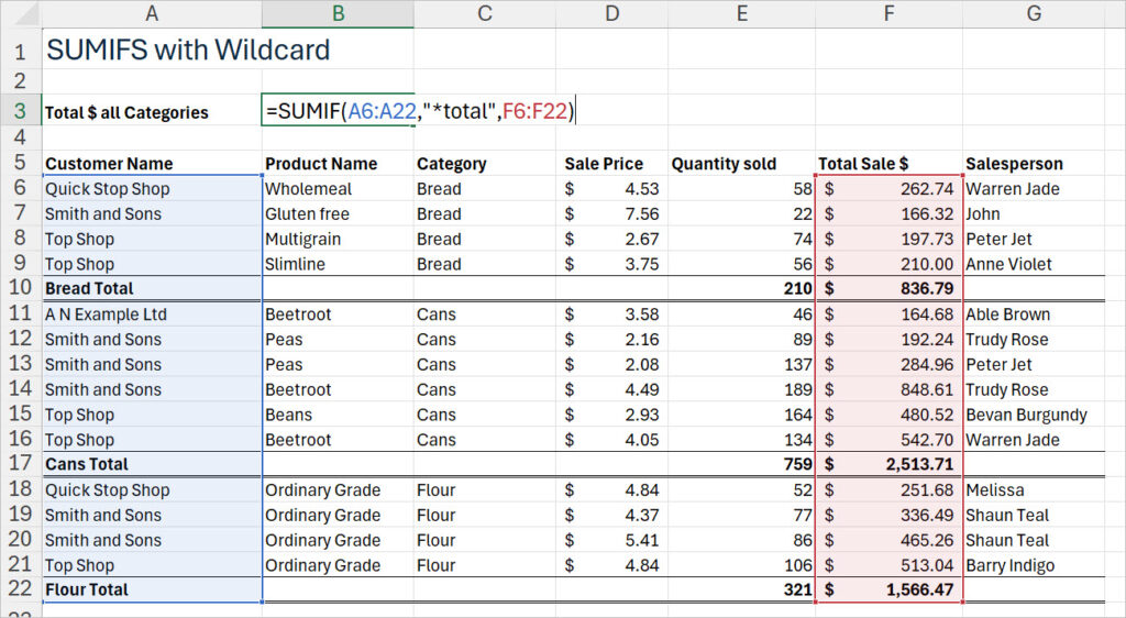
Formula to Total Rows with Partial Matches in Excel

Sometimes the text in your data isn’t tidy. Perhaps your imported file includes row labels such as “Bread Total,” “Milk Total,” and “Cans Total.” Instead of writing separate SUMIFs, you can use a wildcard to tell Excel: “Find anything that ends with the word Total.”

What’s a wildcard?

• * (asterisk) means “match any number of characters.”
• Example: “*Total” finds Bread Total, Milk Total, and Cans Total.
• Example: “A*” finds any text starting with A (like Apples, Apricots).
• ? (question mark) means “match exactly one character.”
• Example: “Jo?n” matches John and Joan, but not Jonathan.

Steps:

1. Click the cell where you want the result.
2. Type =SUMIF(
3. Select the criteria range (e.g., A6:A22).
4. Type a comma, then enter a wildcard pattern (e.g., “*Total”).
5. Type a comma, then select the sum range (e.g., F6:F22).
6. Close the bracket and press Enter. Excel will only total rows where the criteria ends with the word Total.

Formula to Multiply Two Columns and Get the Total (SUMPRODUCT)

SUMPRODUCT is like a smarter version of SUM — it takes two columns of numbers—like “Sale Price” and “Quantity Sold”—and for each row, it multiplies the numbers together. Then, it adds up all those results to give you a single total.

In the example below:

• For each product, Excel multiplies the Sale Price by the Quantity Sold (so you get the total sales for that product).
• Then, it adds up all those totals to show you the grand total sales for everything.

It’s like:
If you sold 3 apples at $2 each, and 5 oranges at $4 each, SUMPRODUCT would do:
(3 × $2) + (5 × $4) = $6 + $20 = $26

Steps:

1. Click the cell where you want the result.
2. Type =SUMPRODUCT(
3. Select the first range (e.g., H8:H25).
4. Type a comma, then select the second range (e.g., I8:I25).
5. Close the bracket and press Enter.

Want to see more SUMPRODUCT examples and tips? Check out my step-by-step guide: How the SUMPRODUCT formula in Excel can help you work more efficiently

Which Formula for Total Should I Use?

Each function has its own strength:

• SUM → Quick totals for rows/columns
• SUBTOTAL → Totals that update with hidden data or filters
• SUMIF → Totals with one condition
• SUMIFS → Totals with multiple conditions
• SUMIF + Wildcards → Totals with flexible text patterns
• SUMPRODUCT → Totals across multiple columns without helper columns

💡 Pro Tip: If your SUM formula isn’t working, check for hidden rows, filtered data, or circular references. For even better results, use SUBTOTAL with filtered lists.

Formula for Total in Excel FAQ’s

Q: What is the formula for total in Excel?
A: The most common way to total numbers in Excel is with the SUM function. It adds numbers in a row, column, or range.

Q: Can I total numbers in Excel without a formula?
A: Yes! If you need a quick answer — for example, checking sales before a meeting — you can highlight the numbers and look at the Sum value in the status bar at the bottom of Excel. It will show the total instantly.

Q: How do I total rows and columns at the same time?
A: Highlight your block of data plus one empty row and one empty column, then from the Home tab, click Sum or press Alt + =. Excel will insert totals for all rows and all columns at once.

Q: What’s the difference between SUM and SUBTOTAL?
A: SUM adds all numbers, even hidden ones. SUBTOTAL only adds visible rows.

Q: What is SUMIF used for?
A: SUMIF totals numbers that match a single condition. For example, you can add sales for just one customer.

Q: How do wildcards work with SUMIF?
A: Wildcards help when your text isn’t exact. For example, you can total all rows ending in ‘Total’ by using “*Total” as the sum criteria argument.

Q: What is SUMIFS used for?
A: SUMIFS is like SUMIF, but lets you apply multiple conditions. For example, total sales for ‘Top Shop’ AND ‘Peach’.

Q: Can I total across multiple sheets?
A: Yes, use a 3D SUM formula.

Q: What if my SUM formula isn’t working?
A: Check for circular references. Check the troubleshooting tips above.

Q: When should I use SUMPRODUCT?
A: Use SUMPRODUCT when you need to multiply two or more ranges together and then total the results. For example, multiplying cost × quantity for sales without creating an extra helper column.

Excel Practice File Download

Conclusion & Next Steps

Excel offers many ways to total numbers — the key is knowing which one to use in each situation. Whether you’re preparing for a job interview, analysing sales data, or simply keeping a tidy budget, these formulas will help you work faster, avoid mistakes, and look confident with your skills.

👉 Try it yourself: Download the practice workbook and test these formulas.
👉 Learn more: Explore my step-by-step Excel online courses for deeper learning.