Excel is famous for its impressive abilities, like handy shortcuts and user-friendly tricks. One of these gems is the Excel double-click feature within spreadsheets.
Double-clicking in Excel isn’t just any click; it’s time-saving and can make your Excel experience much smoother. In this blog, we’ll show you exactly why the double-click is such a game-changer, making Excel easier and more efficient.
In this post, we’ll explore five fantastic ways the double-click feature in Excel can make your tasks smoother and your work more efficient.
1. Hide or Display the Ribbon using Excel double click
The Ribbon in Excel is super handy when navigating through Excel, but it takes up a bit of screen real estate, and sometimes you need more space to see your data. For example, if you are travelling and only have your laptop to work on, this option makes it easier to look at and move around your worksheet.
Double-clicking on any of the tabs in the Ribbon (like “Home” or “Insert“) can hide or display the Ribbon. This is particularly handy when you want to focus on your worksheet without distractions.


Note: Your Ribbon will drop down when you click on a tab and you will then be able to use it but it will also hide again once you are finished using it.
To unhide the Ribbon, double-click one of the tabs on the Ribbon again. The Ribbon will now be visible all the time.
2. Adjust Column Widths using Excel double click
Have you ever encountered that frustrating moment when your text gets cut off because the column is too narrow? For example, in the image below, the title “Retail inc Tax” is cut off.

Double-clicking in Excel can help adjust the column width to the right size without having to click and drag or try to adjust the columns yourself. To adjust the column width so that the header fits within the column:
1. Move your mouse to the edge of the column header (the letter above the column). Once your mouse reaches the end of the column header, a black cross should appear.

2. Once you see the black cross, double-click the edge of the column header. This will adjust the column width to fit your content, as the column will resize to fit the widest entry in that column.

The title “Retail inc Tax” now fits perfectly within the column.
Note: Double-clicking the edge of the column header will save you space, as the column width will adjust to only the widest entry. In other words, if the column entries have extra space in the cells, double-clicking the edge of the column header will remove this extra unneeded space. This is extremely useful for when you want to print and notice a column is moving off onto another page, as this option saves space and may allow the entire spreadsheet to fit on the one printed page.
3. Double click for in Cell Editing in Excel
Editing cells is a fundamental Excel task, and the double-click feature allows you to insert, delete and change data within these cells straight from the cell source.
1. Locate the cell you want to edit. For example, if we wanted to edit cell F4.

2. Double-click any cell you want to edit, and you’ll be able to modify its contents directly without the need to navigate to the formula bar or press F2. The cell will be ready to edit when you see the insertion point flashing within the cell.

3. Type in the information you want to add to the cell.

4. Press Enter, and the new information will be added to that cell.

The cell will now have the new information in it.
4. Copy to the Bottom of a Column using Excel double click
Imagine copying data down a column without repetitive copying and pasting or dragging to the bottom. The double-click in Excel allows you to do this which saves so much time.
For example, in the image below, we entered data into cell F4.

To copy information down the column, try these steps:
1. Locate the tiny square at the bottom-right corner of the cell you have entered data into (it’s called the “fill handle”).

2. Hover your mouse over the fill handle. Your mouse should look like a little black cross when hovering over the fill handle. In this example, we hover our mouse over the tiny square in the bottom-right corner of cell F4.

3. Double-click the tiny square, and Excel will automatically copy that data down to the last adjacent cell with content.

This tip is super handy when you have many rows that need to be filled in. For example, if there are 2000 rows, using this trick will save you a lot of time.
5. Instantly Insert and Rename Worksheets using Excel double click
Managing multiple worksheets is a breeze with the double-click feature.
To quickly insert a new worksheet and rename simultaneously, follow these steps.
1. Double-click the plus (+) icon at the bottom of the screen in the worksheet tabs.

2. The worksheet title should now be highlighted with the insertion point inside.

3. Type the new title and press Enter.

The worksheet should now be renamed with the new title.
Additionally, renaming an already established worksheet is as easy.
1. Double-click the worksheet tab at the bottom and type the new name.

2. Hit Enter.

Your worksheet will now be renamed to the new title.
Watch the Excel Double-Click Tips Tutorial
[Watch on YouTube] / [Subscribe to our YouTube Channel]
Conclusion
The double-click feature is a simple way to save time when working in Excel. It makes it easier to read and view your workspace and minimises the time it takes to complete essential tasks. So, save these tips to try in your next Excel session.
Was this post helpful? Let me know in the comments below.
Want to Learn Excel Properly?
Join the Excel at Work Learning Hub
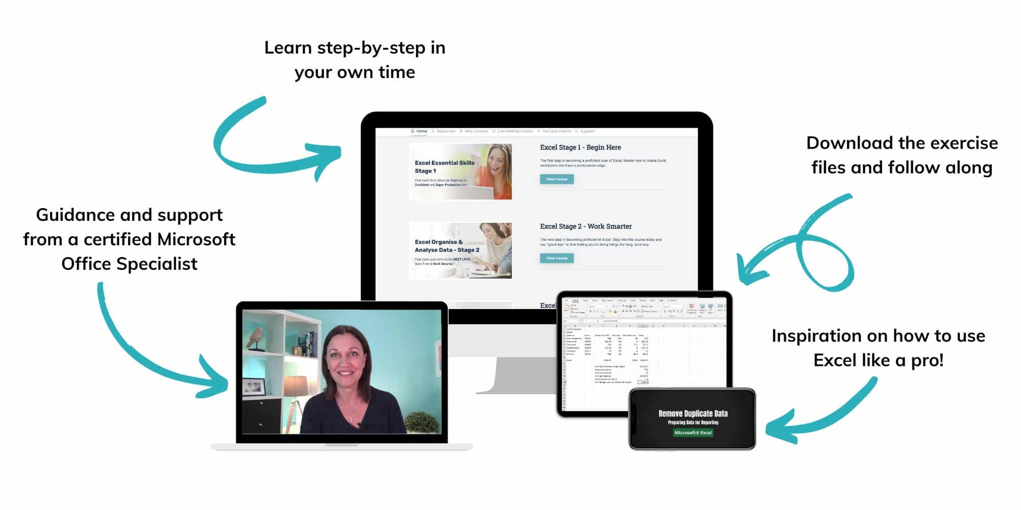
The Excel at Work Learning Hub is an online self-paced Excel training membership designed for people who use Excel at work—in offices, on sites, in schools, in small businesses, and everywhere in between.
Go from Beginner to Confident – Guaranteed!
Only $59NZ /month
Cancel anytime • No pressure • 14-day 100% Money Back Guarantee

Certified Microsoft Office Specialist
Was this blog helpful? I’m here to empower your journey with Excel, aiming to make your daily tasks more efficient and boost your potential.
Share your thoughts in the Comments below – your insights not only enrich others, they also help me tailor future content to your needs.
And if you’re looking to take a step further, join our exclusive ‘Insider Group‘. As a member, you’ll receive Weekly Super-Tips, and early access to in-depth tutorials. Sign up Today!
Happy Excel-ling!!