How to copy and paste visible cells only in Excel (excluding hidden rows and columns)

Learn how to copy and paste, excluding hidden columns or rows in Excel.

Ever tried to copy and paste data thinking you will be pasting, excluding the hidden columns or rows only to have the hidden data copied too?

Copying a data range that contains hidden data can be challenging when the hidden data travels with the copied range.

In this post I’ll explain how to copy and paste the visible cells only – hidden cells are excluded.

Why does Copy and Paste include hidden data in Excel?

Let’s look at what happens when we try to copy and paste a range with hidden data. In the example below we have an Excel spreadsheet with information on sales.

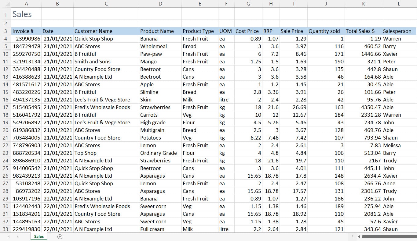
In this example, we are wanting to hide rows 6-9 and copy and paste the information in this data set without these rows included.

To follow along, rows 6-9 have been highlighted in yellow so that they are easily identified as we continue through the steps.

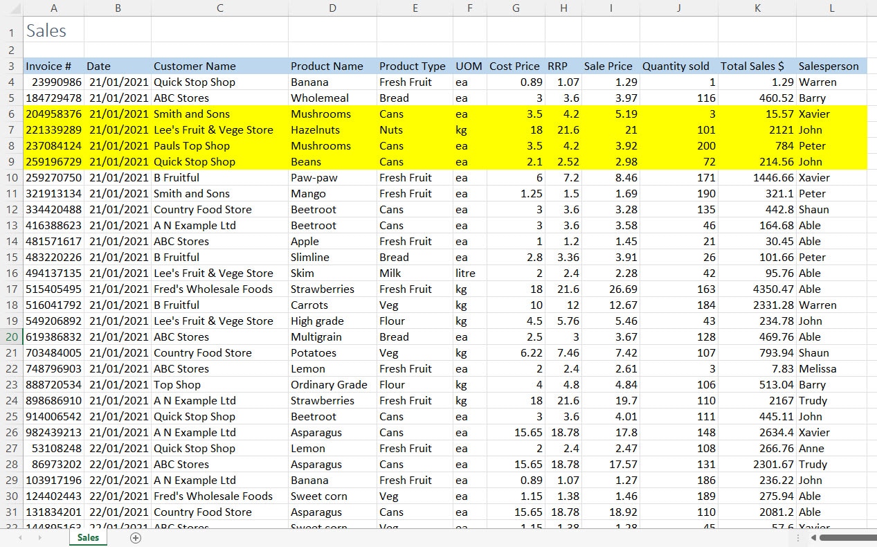
To hide these rows, we will do the following.

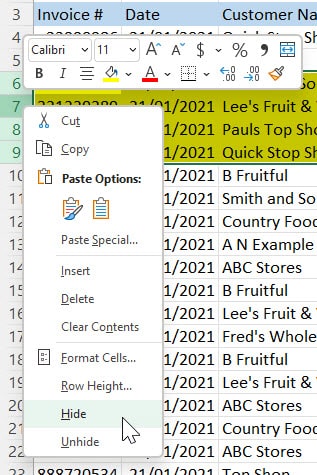
Step 1: Select the rows we want hidden by clicking and dragging over the row numbers. In our example, this is rows 6-9.

Step 2: Right-click the selected rows and then select Hide from the menu.

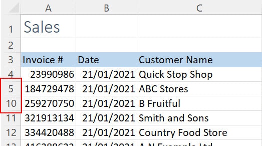
The rows we have selected will now be hidden.

You can see in our example, rows 6-9 are hidden. We can easily identify this as the highlighted rows are now hidden and the row numbers jump from 5 to 10.

Copying data that has hidden rows

Now let’s try copying the first 3 columns of data in this table to another worksheet. We are assuming that the hidden data will not copy because it is hidden.

Step 1: We will select the data range that we want to copy, including the hidden rows. In this example, we want to copy the Invoice number, Date and Customer Name columns.

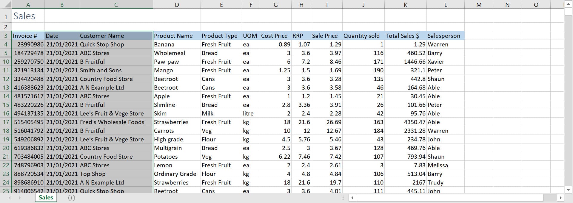
Step 2: To copy the range we’ve selected, we will right-click the selected range and select Copy from the shortcut menu (or press Ctrl + C).

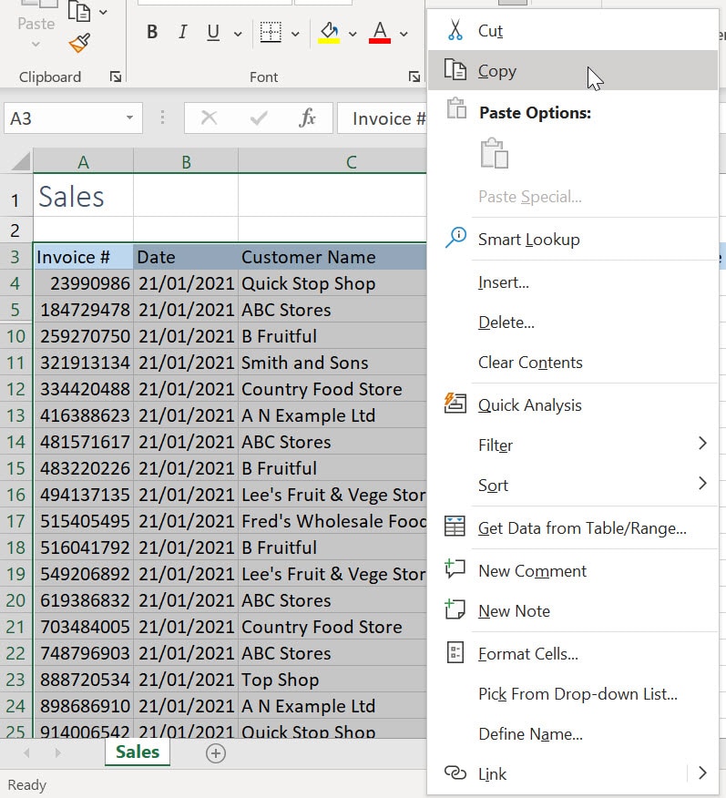
Step 3: We will now go to where we want to paste the data and select the cell that will be the top, left cell of the pasted range. In our example, we created a new sheet and are now wanting to paste the copied data into cell A3. The name of our new sheet is Sheet1 as this was the default name given to the sheet by Excel.

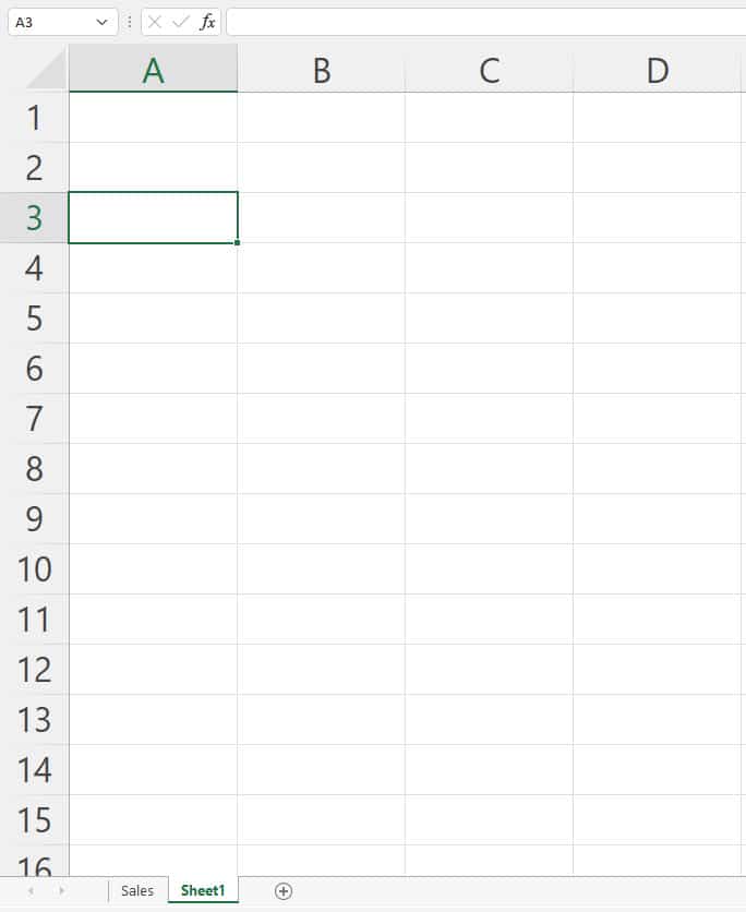
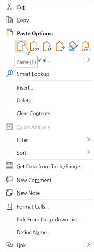
Step 4: We will now paste the copied data by doing a right-click and selecting Paste from the shortcut menu (or we can press Ctrl + V).

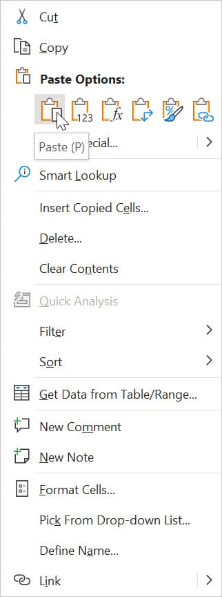
Step 5: Unfortunately, we can see that the hidden data has been copied and included when we paste. This is easily identifiable as you can see the rows we highlighted in yellow, prior to doing the copy, have also copied over.

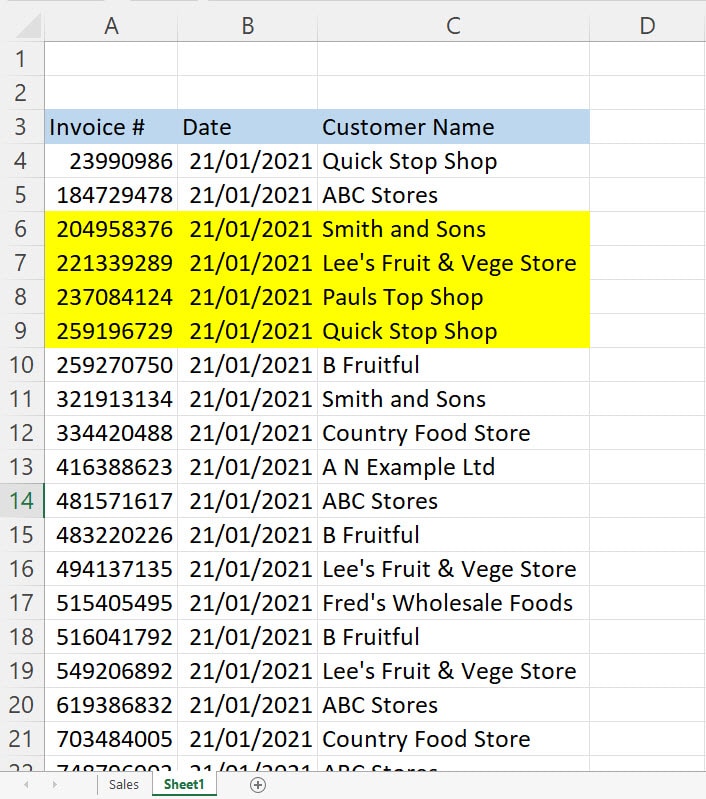
This is because when we selected the data to be copied in Step 1, we are actually selecting both visible AND hidden data.

Therefore, when we copied we are copied ALL the data, not just the visible cells.

Most of the time this is not ideal, and you don’t want these hidden rows to travel over with the data you are copying and pasting.

The following steps will teach you how to paste visible cells only in Excel, excluding any hidden rows or columns.

Copying and pasting visible cells only in Excel (excluding hidden cells)

Step 1: Start by selecting the area you want to copy. In our example we will select the Invoice, Date and Customer Name columns. The highlighted rows 6 to 9 are hidden.

Step 2: From the Home tab, select Find & Select.

Step 3: Select Go To Special.

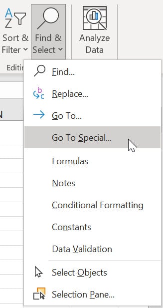
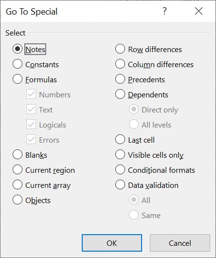
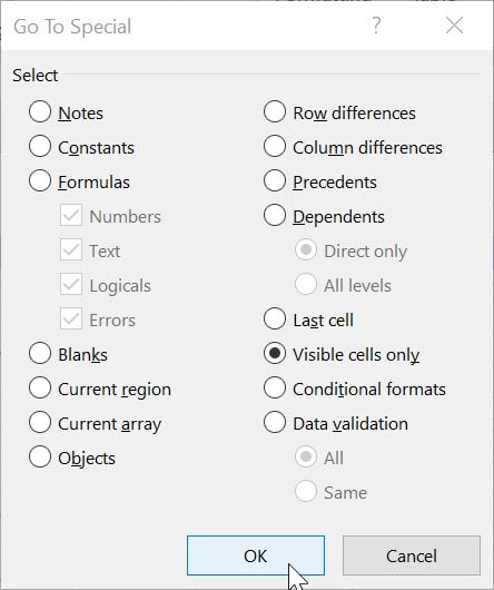
The Go To Special dialogue box will appear.

Step 4: Select Visible cells only. This ensures only the visible cells are included in your selection. The hidden cells are excluded.

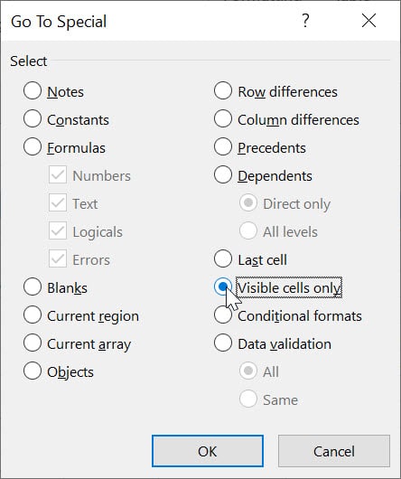
Step 5: Click OK.

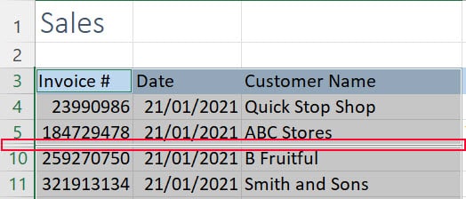
You will now see that the visible cells have been selected and the hidden cells are excluded. A small line within the selected area shows this .

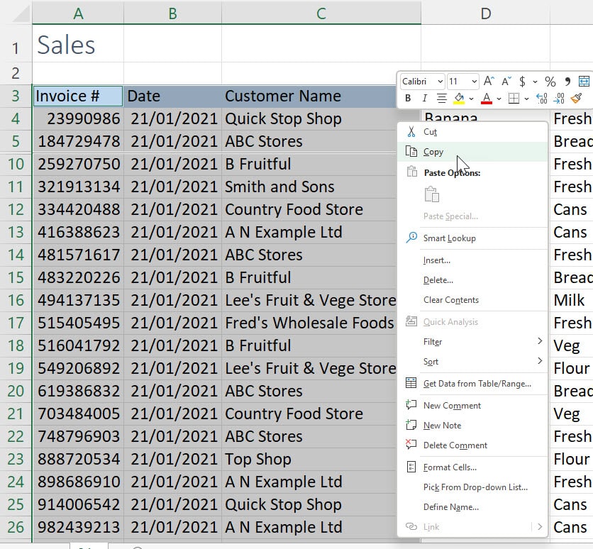
Step 6: Now Copy the selected cells by right-clicking over the selected area and selecting Copy from the shortcut menu (or press Ctrl + C).

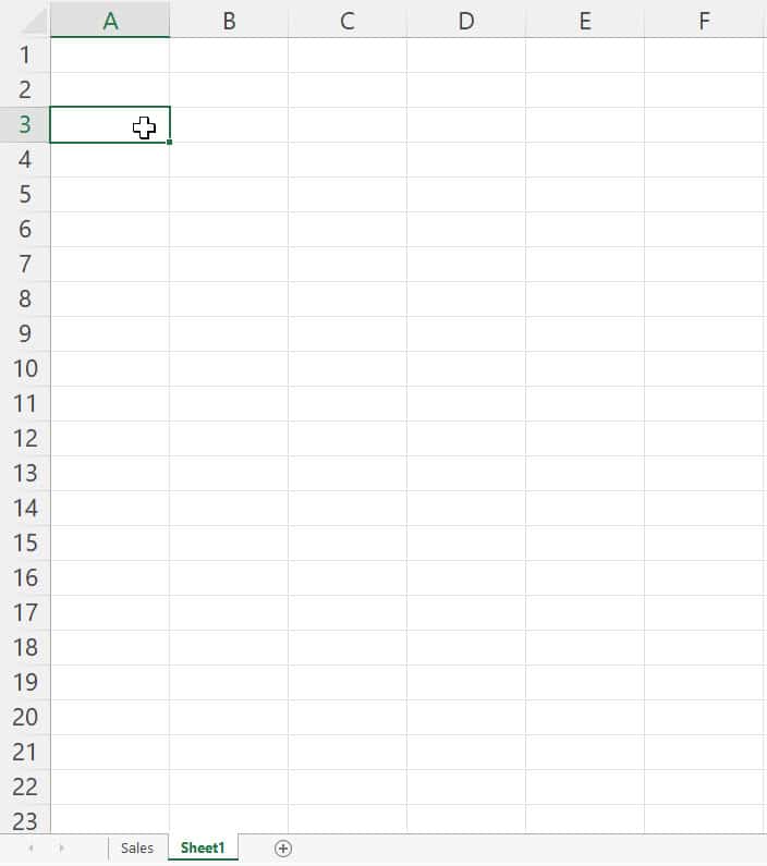
Step 7: Go to where you want to paste the data and select the cell that will be the top, left cell of the pasted range. In our example, we created a new sheet called Sheet 1 as this is the default name given by Excel and we selected cell A3.

Step 8:Paste by doing a right-click and selecting Paste from the shortcut menu (or press Ctrl + V).

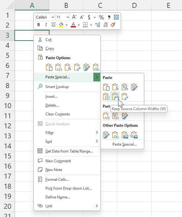
Super Tip: If you want to paste your cells with the exact same column widths as the sheet they were copied from, when you go to paste do a right-click and select Paste Special. From there, select Keep Source Column Widths (W).

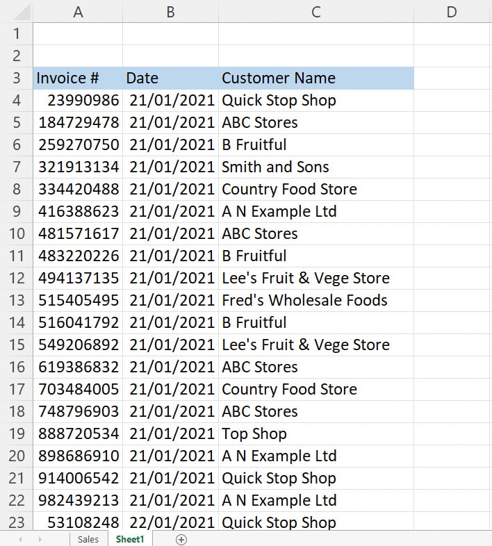
Only the visible cells will be pasted.

In this example, we can easily tell that only the visible cells have been pasted as the hidden rows were highlighted in yellow and they have not appeared.

Excel Shortcuts for Copying and Pasting visible cells only (excluding hidden cells)

1. Select the range to be copied, including the hidden data.

2. Press ALT + ; (ALT + semicolon to select only visible data and exclude any hidden data)

3. Press Ctrl + C (to copy)

4. Go to where you want to paste the data and select the cell that will be the top, left cell of the pasted range.

5. Press Ctrl + V (to paste the data).

Watch the Excel Copying and Pasting Ranges with Hidden Cells Tutorial

[Watch on YouTube] / [Subscribe to our YouTube Channel]

To Sum up

The trick is to ensure you are only selecting visible cells prior to doing your Copy.

Once you have this mastered you can easily control your data and copy visible cells only.

Was this blog helpful? I’d love to know. If you’re a beginner or if you use Excel every day please let me know if I helped in some way by leaving a comment below.