Filters within Microsoft Excel are like magic wands as they allow you to sift through vast amounts of data effortlessly. But what if I told you there’s a way to make this process even quicker and more efficient? Well there is, with the use of Excel filter shortcuts and these shortcuts are the secret to optimising your data filtering.
In this blog, we will equip you with the knowledge to send you on your way to becoming an Excel filter shortcut expert. We will uncover 6 different Excel filter shortcuts that will save you time and simplify your data analysis. Whether you're new to Excel or a pro, get ready to boost your data filtering skills.
- Basics of Excel Filters
- Common Filter Tasks
- Excel filter shortcut #1: Turning AutoFilter on and off
- Excel filter shortcut #2: Filtering on selected data ranges
- Excel filter shortcut #3: Displaying the Filter menu
- Excel filter shortcut #4: Selecting options from the Filter menu
- Excel filter shortcut #5: Underlined letters in the Filter menu
- Excel filter shortcut #6: Clear/remove all filters
Basics of Excel Filters
Think of Excel filters as your data's GPS, guiding you to the exact information you need. These shortcuts allow you to sift through mountains of data to find what’s relevant.
How to access the Filter in Excel
To activate your Filter in Excel:
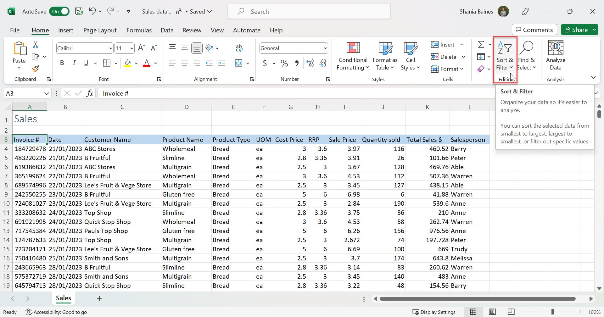
1. Select ALL of the data to be filtered, including the heading row.
2. On the Home tab, select Sort & Filter.
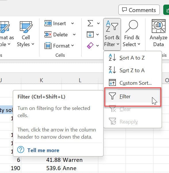
3. From the drop-down menu select Filter.
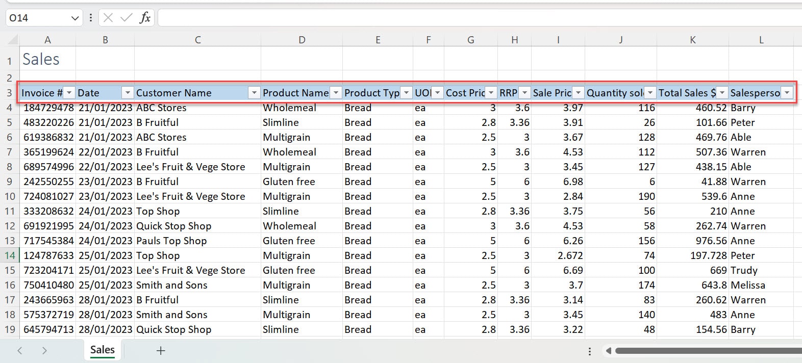
Filter drop-down arrows
Once you've turned on filters, you'll spot small drop-down arrows in each column header with data.
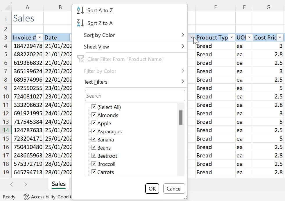
Click on one, and you'll reveal a menu of filtering options. This is also known as the Filter menu.
Common Filter Tasks
In this section, we'll explore common filter tasks and the handy shortcuts that make these tasks a breeze.
Excel filter shortcut #1: Turning AutoFilter on and off
Shortcut: Ctrl + Shift + L
Ctrl + Shift + L is the shortcut to instantly turn on your filter. If you want to turn your filter off, press Ctrl + Shift + L again and it will instantly be turned off.
Note: Turning off AutoFilter will remove all the filtering on your data.
Excel filter shortcut #2: Filter only selected columns
Shortcut: Select the range and press Ctrl + Shift + L
This shortcut is similar to the AutoFilter shortcut. However, this time it requires you to select only the columns that you want to filter. Here's how you do it.
Note: This example is assuming your data has no empty rows. If your data contains empty rows, you will have to select all of your data’s range and then follow the steps below.
1. Select the column headers for the columns you want to have the filter on. In our example, we want the filter on columns C (Customer Name), D (Product Name) and E (Product Type).
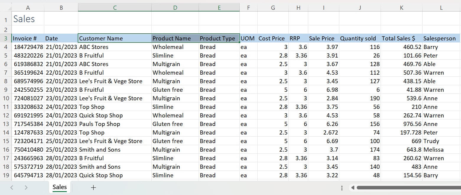
2. Press Ctrl + Shift + L and the filter should be applied only to the columns selected.
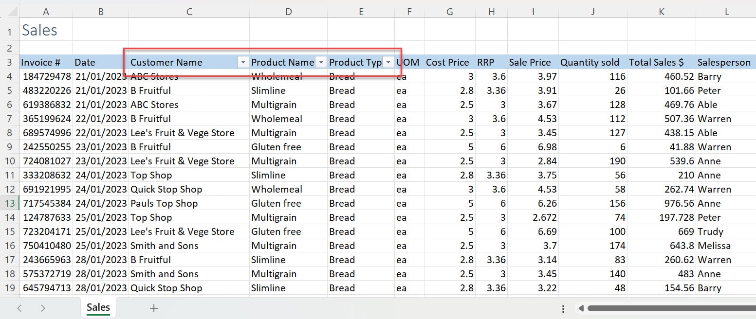
3. To turn them off, select Ctrl + Shift + L again.
Note: If you are wanting to turn filter on for one column only, select all of the data in that column, from the column heading then follow the steps above. Another quick shortcut to select the entire columns data, click on the column heading and then press Shift + Ctrl + Down Arrow.
Excel filter shortcut #3: Displaying the Filter menu
Shortcut: Alt + Down Arrow
One of the most frequently used filtering techniques is narrowing down your data to specific values.
For instance, imagine you have a large dataset of information, and you want to filter only the items with a certain category. In Excel, we do this in the Filter menu. In our example, we want to filter only the items in the Product Type column which is found in column E.
To do this:
1. Ensure filtering is turned on.
2. Select the column header of interest e.g. the header ‘Product Type’ in cell E3.
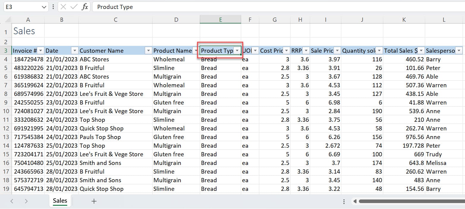
3. Press Alt + Down Arrow, and the Filter menu appears.
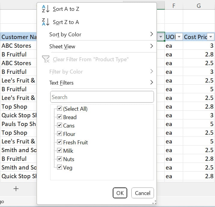
4. From here you can select the option you would like with your mouse, or follow the steps in Excel Filter shortcut #4 to select with keyboard shortcuts.
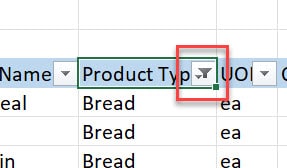
Note: You can identify a column that is filtered as there will be a little filter icon where the filter arrow is on the header of the column.
Excel filter shortcut #4: Selecting options from the Filter menu
Shortcut: Up and down arrows, Enter and Spacebar
While you're in the Filter menu, you can use your up and down arrows to navigate around the menu. These shortcut keys in combination with Enter, which allows you to select an option, and the Spacebar, which allows you to check and uncheck boxes, make it faster to apply the filter options you want.
The following steps show you how to use these shortcut keys. For our example, we want to apply ‘Sort Z to A’ on the Product Name column (in column E) and we want to filter to only look at Almonds, Beetroot, Carrots, Lemon and Nuts.
To do this:
1. Press Alt + down arrow on the Product Type column header to open the Filter menu.
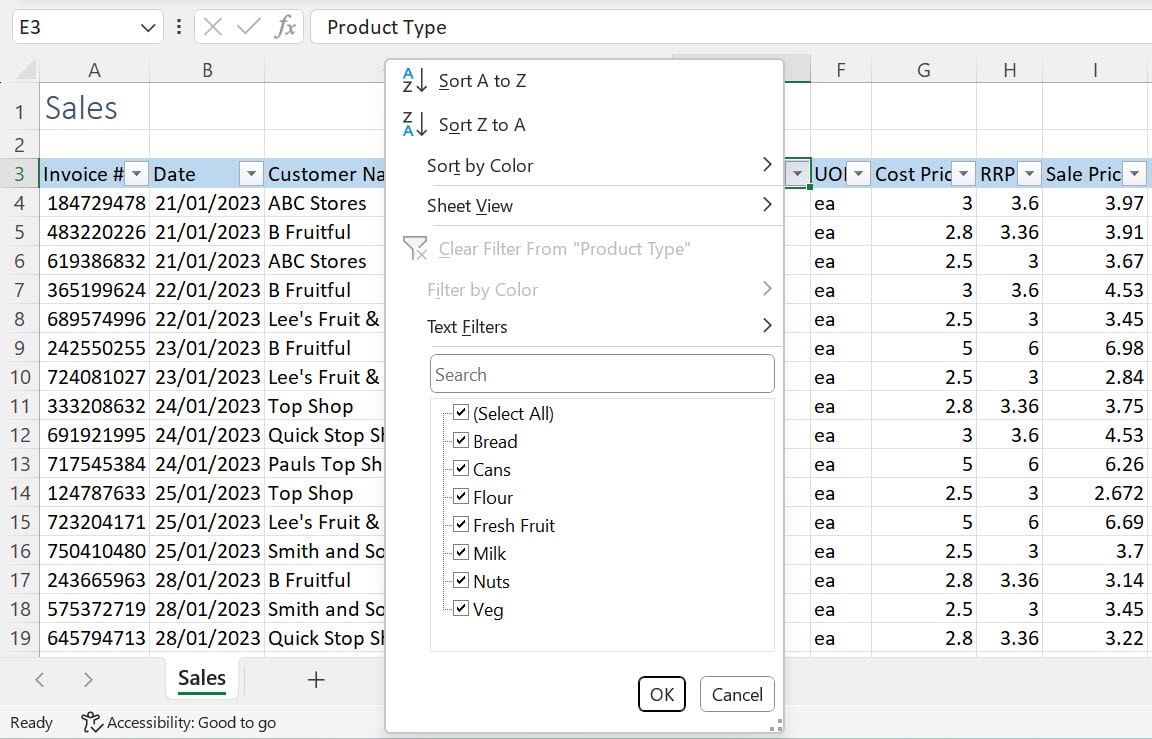
2. With the Filter menu displayed, press your up arrow to move up options in the menu and press your down arrow to move down the options in the menu.
Note: The option that you’re currently on will be outlined in a black box.
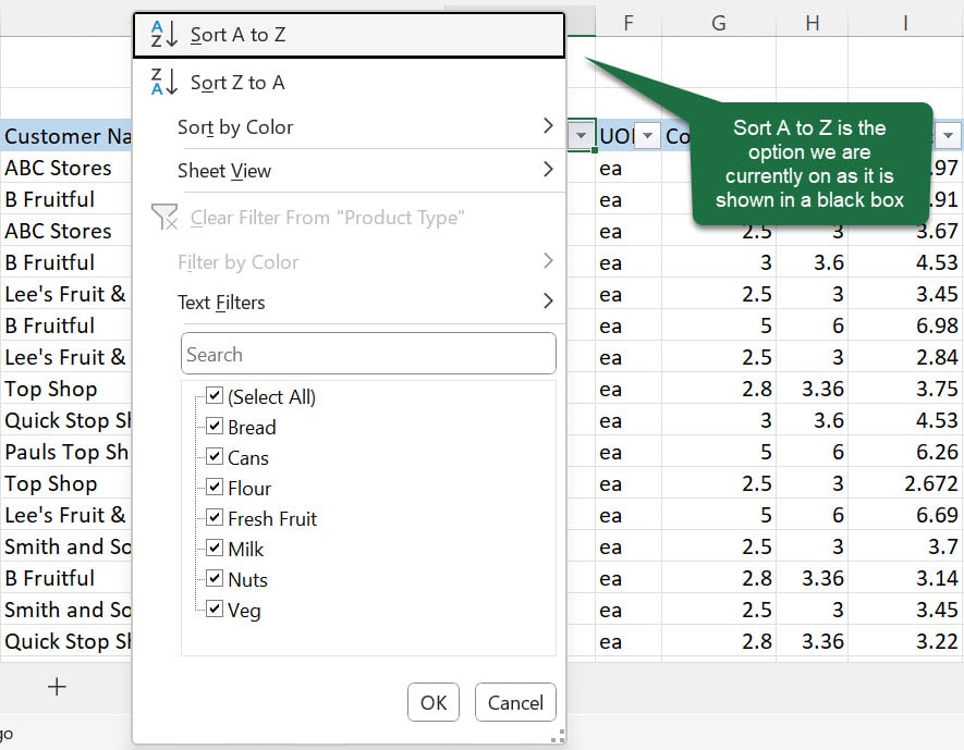
3. Navigate to the option you want to apply. For our example, this is the option ‘Sort Z to A’ on the drop-down menu.
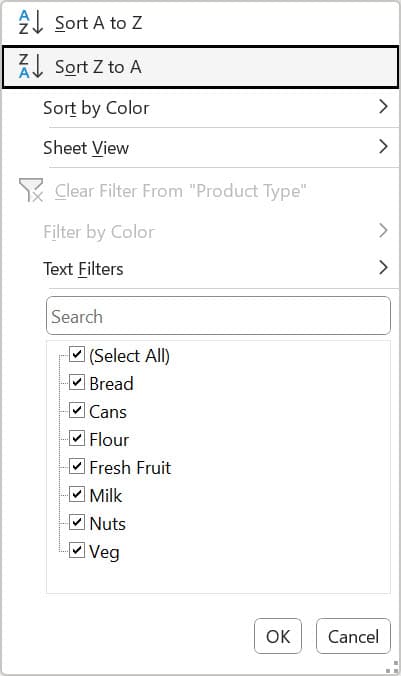
4. Press your Enter key and the option will be applied. Our column should now be sorted in reverse alphabetical order.
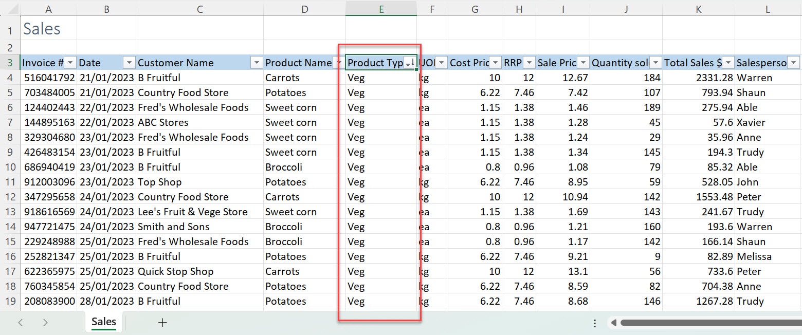
Now, we want to filter the column only to display Bread, Flour and Milk. You can do this by using the Spacebar to check and uncheck boxes in the Filter drop-down menu.
To do this:
1. Press Alt + down arrow on the Product Type column header to open the Filter menu.

2. Navigate to the Filter checked options with your down arrow key.
3. Unselect or select options by pressing your Spacebar key. We want Bread, Flour and Milk all to be checked and everything else unchecked.
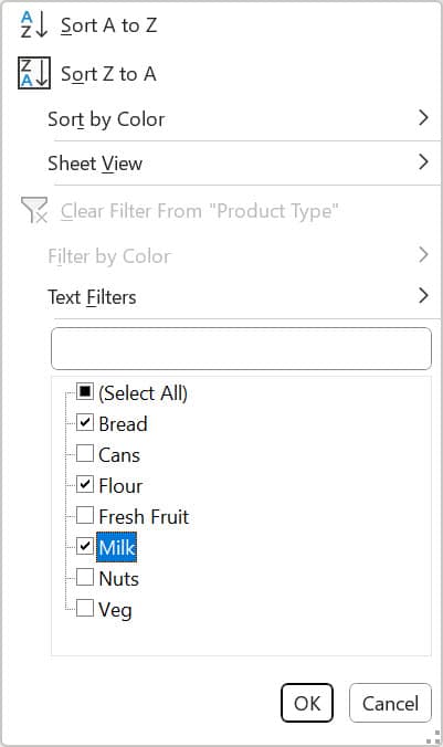
Note: You can unselect ‘Select All’ then select the options you want rather than unselecting all the other options to save you time.
4. Press Enter and the filter should be applied.
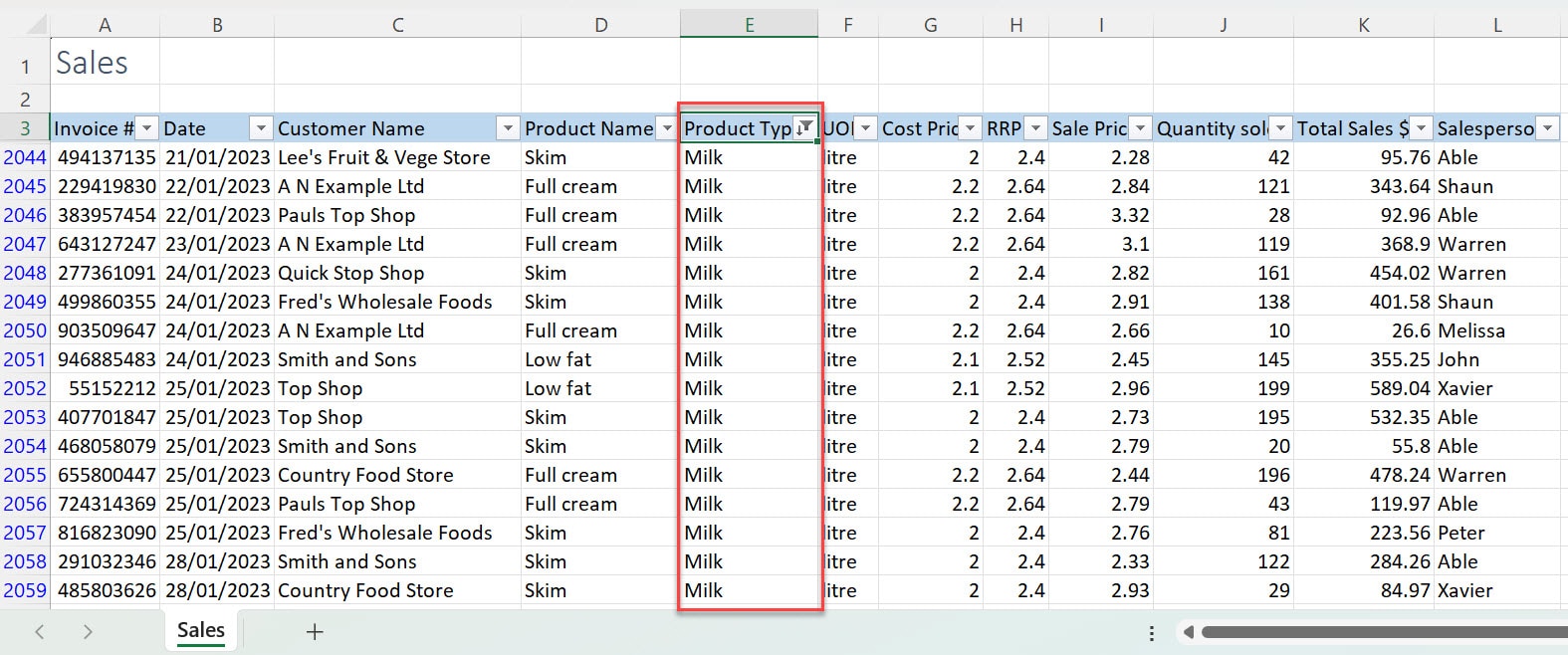
Summary of these shortcuts inside the filter menu
Keyboard Shortcut | What it does |
|---|---|
Up and down arrows | Allow you to move up and down the drop-down menu options |
Enter | Allows you to select the option you are on |
Spacebar | Allows you to check and uncheck boxes within the search box |
Excel filter shortcut #5: Underlined letters in the Filter menu
Shortcut: S, O, T, V, C and F
When inspecting the filter drop-down menu, you can see each option has an underlined letter on it.
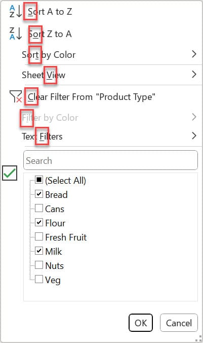
These underlined letters correspond to the key that can carry out that specific option. For example, on ‘Sort A to Z’ there is an underline under the letter S. This means that while in the filter menu, if you press S on your keyboard, it will select the option ‘Sort A to Z’ and your column will be in alphabetical order.
Here is a table depicting what keys do what
Option | Underlined letter and keyboard shortcut | What it does |
|---|---|---|
Sort A to Z | S | Automatically sorts column in alphabetical order |
Sort Z to A | O | Automatically sorts column in reverse alphabetical order |
Sort by Color | T | Opens sub menu for ‘Sort by Color’ |
Clear Filter | C | Automatically clears the filter off selected column |
Text Filters | F | Opens sub menu for ‘Text Filters’ |
Search box | E | Takes you straight to the search box where you can type what you are looking for |
Note: Do not hold any other keys with these shortcuts. Press only the key while in the filter menu and it will carry out its function.
Tip: The sub-menus will also have underlined letters in which you can use to open options further.
Excel filter shortcut #6: Clear/remove all filters
Shortcut: Alt > A > C
We have already covered that Ctrl + Shift + L can turn filters on and off as well as Alt + down arrow followed by C. However, there is also another shortcut that can be used to clear all of the filters on the range of data that is being filtered. This shortcut allows you to remove the filter without removing the filter arrows on your column headings.
The shortcut Alt > A > C can be pressed to remove all of the filters in the filtered range.
To do this:
1. Select a cell in the range of data being filtered. For example, we selected cell E2048.
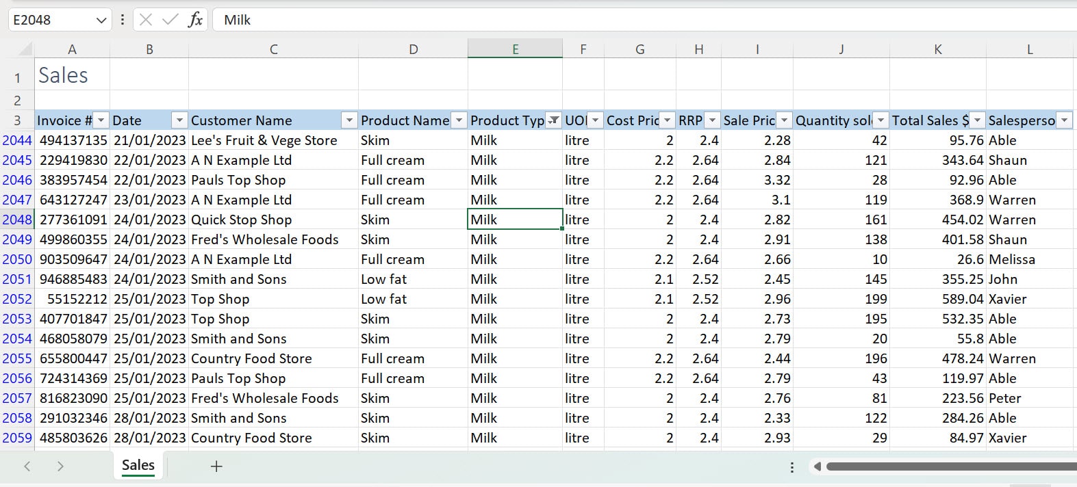
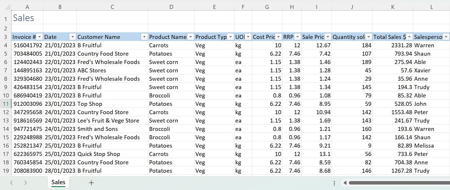
2. Press Alt then A then C. They have to be pressed in order (Alt then A and then C), in order for the shortcut to work. Your filters should now be removed.
Summary of the shortcut keys for Filter
Shortcut key | What it does |
|---|---|
Ctrl + Shift + L | Turns AutoFilter on and off |
Select the range and press Ctrl + Shift + L | Allows for a selected range to be filtered without the rest of the worksheet being filtered |
Alt + Down Arrow | Opens filter menu |
While in the filter menu: | Navigate around the filter menu. Up and down arrows allow you to move up and down the options, Enter allows you to select an option and Spacebar checks and unchecks options in the search box. |
While in the Filter menu: | These shortcut keys correlate to the underlined letter in each option on the filter drop-down menu. The shortcut keys select their corresponding option which has that letter underlined. |
Alt > A > C | Clears all filters on the range. |
Conclusion
These are just a few of the invaluable shortcut keys that can greatly streamline your data-filtering tasks in Excel. Incorporating these Excel filter shortcuts into your workflow will enhance your efficiency and speed when working in Excel.
Was this post helpful? let us know in the Comments below.

