Excel – How do I merge cells within a range that is formatted as a Table?

Question: When I use Excel “Format as Table” to format a range, the Merge & Center button is greyed out and becomes inactive and I can no longer merge cells.

Answer: This is because the cells are within an Excel Table format, and we are unable to merge cells within a Table format.

However, there is an alignment format you can use to give Table formatted cells the look of a merged cell.

Why Can’t I Merge Cells in an Excel Table?

In the example below I’m wanting to merge the text ‘Status TBC’ across two cells. However, the Merge and Centre button is greyed out and no longer available.

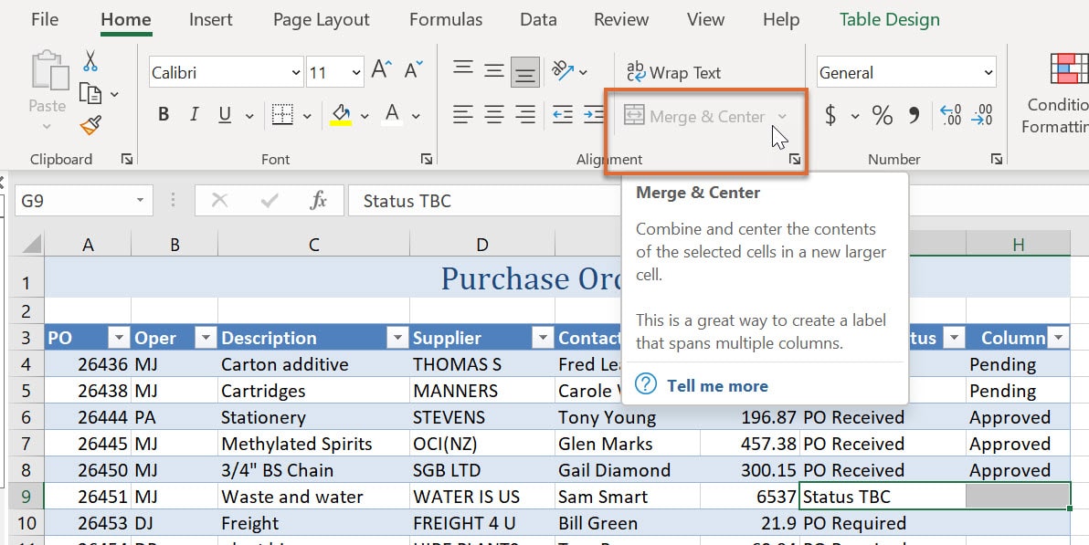
Excel spreadsheet with Merge & Center button on Excel ribbon greyed out and shown in a red box

In this blog post I’m going to give you a work-around for when the Merge & Center button is greyed out, and cover steps that you can take to give your Table cells the look of a merged cell.

1. Convert the Table to a Range

The first thing I need to do is remove the Table functionality from my data.

Warning: the following steps will leave the formatting on your Table but will remove all Table functionality so please proceed with care.

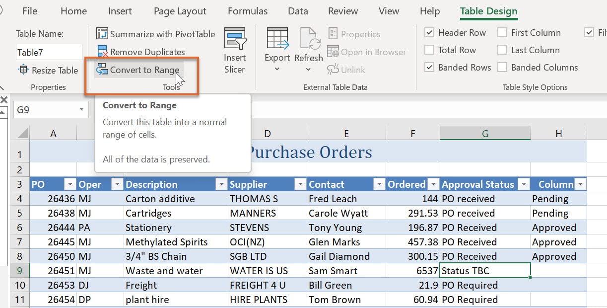
1. To do this select any cell within the Table area and then click the Table Design tab.

2. Click the Convert to Range button.

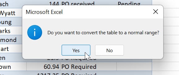
Excel spreadsheet in the Table Design tab with the Convert to Range option shown in a red box

3. Excel will ask ‘Do you want to convert the table to a normal range. Click Yes.

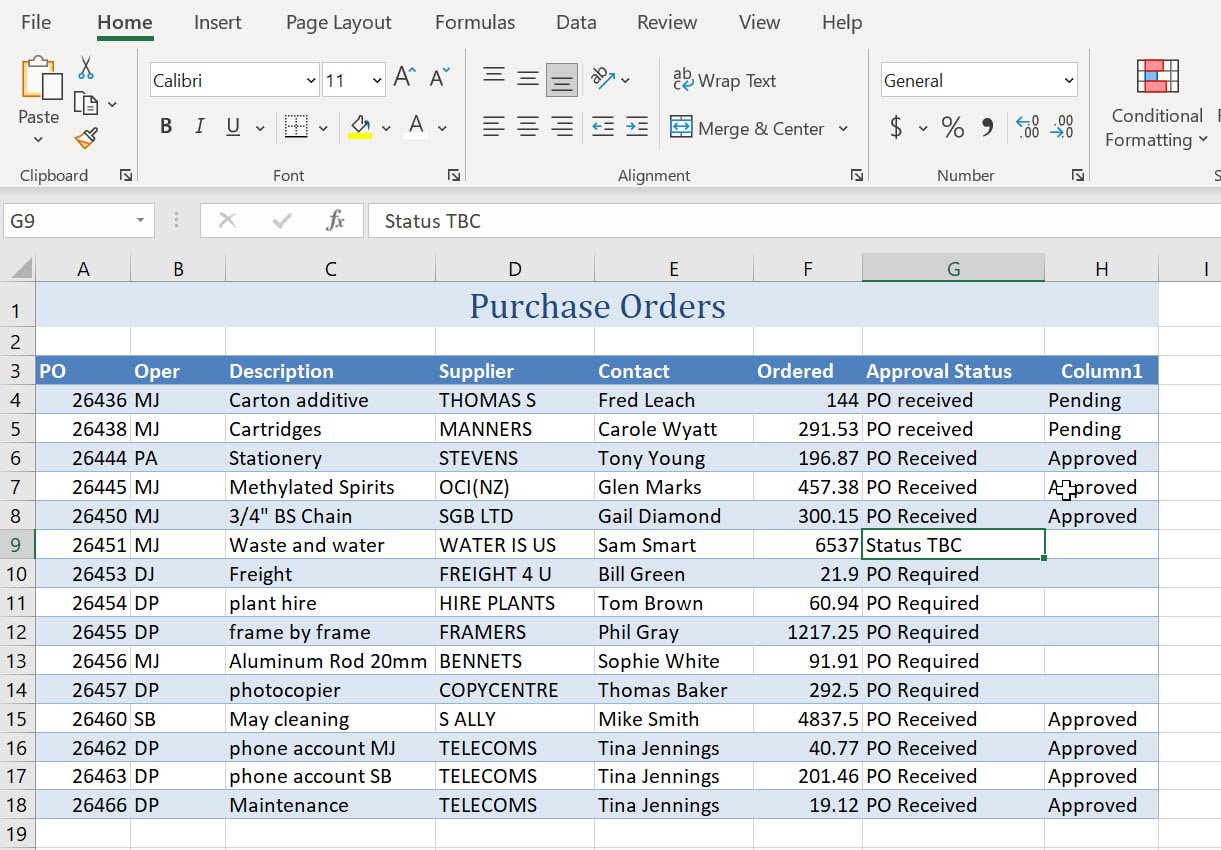
Microsoft Excel box saying Do you want to convert the table to a normal range? The mouse is selecting the option Yes

4. Your Table will now be converted back to a normal range. The formatting will remain, but all other Table features will be removed.

2. Apply Center Across Selection

Now that the Table has been removed you will now be able to use an alignment setting called Center Across Selection. This format allows us to give the cells a merged look.

Note: the next steps will work for data inside the Table, but not for Table headings. Please see Merging Table headings doesn’t work below.

1. First select over the cells that you would like to merge. In the example below I have selected over cells G9 and H9.

2. Click the small arrow in the bottom right corner of the Alignment group.

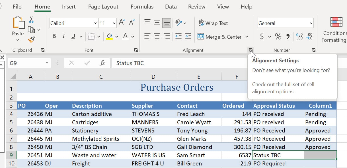
Excel spreadsheet in the Home tab with the alignment settings button being selected by the mouse

3. This will open the Format Cells dialogue box with the Alignment tab settings displayed.

4. From the Text alignment, Horizontal options box select Center Across Selection.

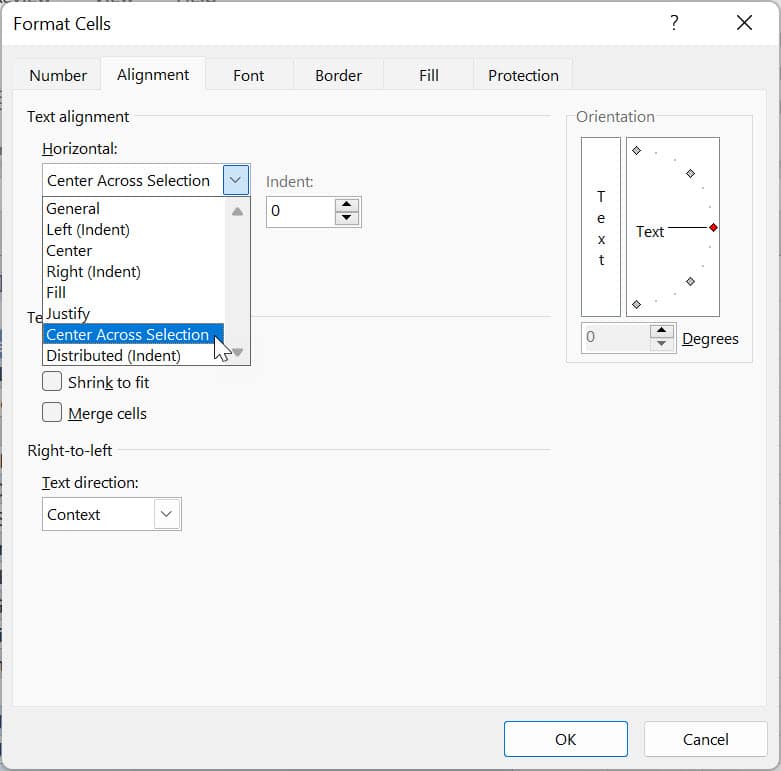
Format Cells dialogue box in the Alignment tab. Under Horizontal: Center Across Selection is being selected.

5. Click OK.

6. It will now appear that the cells have been merged.

Excel spreadsheet with PO, Oper, Description, Supplier, Contact, Ordered, Approval Status and Column 1. One row in Approval Status and Column 1 has Status TBC shown in red box.

7. Even though the cells look to be merged they still are separate. The text ‘Status TBC’ still resided in cell G9. The Center Across Selection option gives the look of a merged cell, without you needing to merge the cells.

Purchase Orders spreadsheet with cell G9 selected where it says Status TBC.

3. Select the data and use Format as Table again

8. Now I will insert a Table over the data once more. To do this I will select the data and then from the Insert tab click Table.

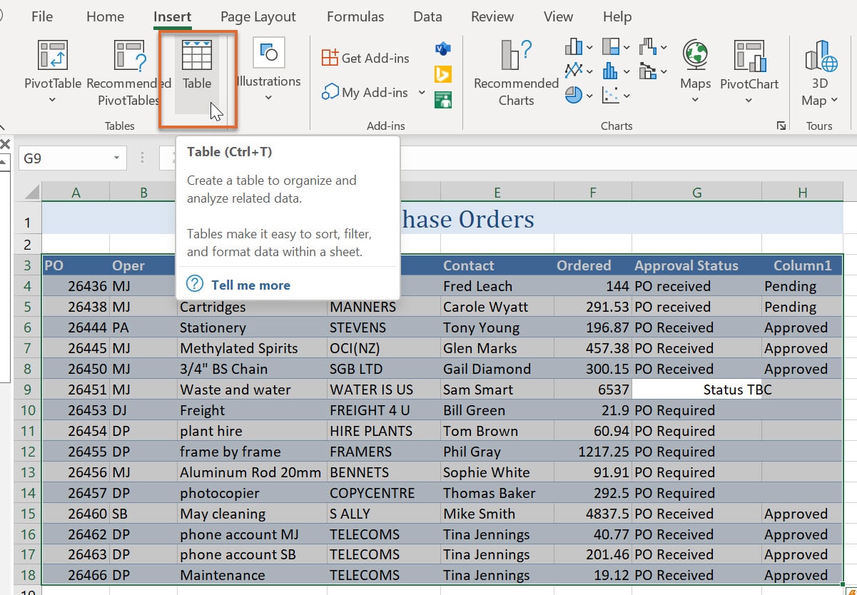
Excel Insert tab with the Table option shown in a red box.

9. Excel will ask if I wish to create a Table. Click OK.

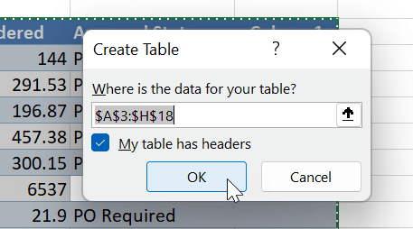
Create a Table dialogue box with $A$3:$H$18 in the Where is the data for your table? and the My table has headers box is selected with the mouse pointing towards OK

10. A Table will be applied over the data once more and the cells formatted with Center Across Selection will still have the look of a merged cell.

Excel spreadsheet with columns PO, Oper, Description, Supplier, Contact, Ordered, Approval Status and Column. Status TBC is merged in the two columns Approval Status and Column.

Please note: if you will be using the Filter or Sort features within the Table format, content that has been formatted using Center Across Selection will be included in the column it was originally entered into.

Merging Table Headings doesn’t work

In my example below I have used the Centre Across Selection format to merge two column headings. The cell containing the text ‘Approval Status’ now has a merged look.

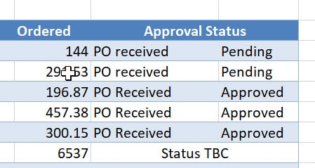
Ordered column and Approved Status column. Approval Status is the title for the two columns beneath.

With the cell formatted using the Centre Across Selection I can insert a Table over the data.

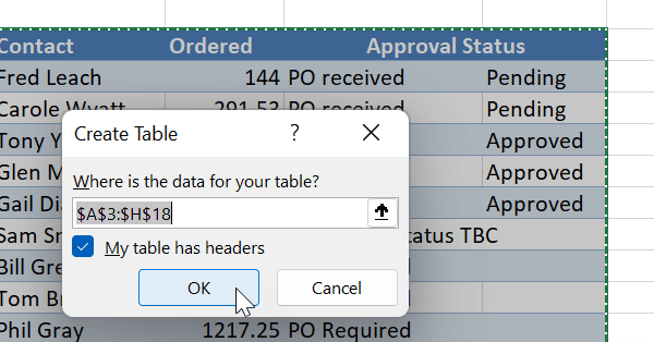
Create a Table dialogue box. In the Where is the data for your table? there is $A$3:$H$18. The My table has headers box is selected and the mouse is pointing towards OK

However, as soon as I insert a Table over the data, Excel will give me a new column heading, ‘Column1’.

The merged cells with ‘Status TBC’ inside the Table remain with the merged look, but the ‘Approval Status’ is reset.

Purchase Order spreadsheet with columns Approval Status and Column shown in a red box and the cell Status TBC also shown in a red box.

This is because each column within a Table requires a unique heading, therefore Centre Across Selection will not work for cells in the heading row.

To Sum up

Using this quick work around in Excel to give your formatted Table cells the look of merged cells.

Was this blog helpful? I’d love to know. If you’re a beginner or if you use Excel every day please let us know if we helped in some way by leaving a comment below.

If you enjoyed this and want to learn more about how to use Excel, have a look at our posts How to copy and paste visible cells only in Excel (excluding hidden rows and columns) and How to Sum only visible cells in Excel when using Filter.

**Sharyn Baines**
Certified Microsoft Office Specialist

Was this blog helpful? I’m here to empower your journey with Excel, aiming to make your daily tasks more efficient and boost your potential.

Share your thoughts in the Comments below – your insights not only enrich others, they also help me tailor future content to your needs.

And if you’re looking to take a step further, join our exclusive ‘Insider Group‘. As a member, you’ll receive Weekly Super-Tips, and early access to in-depth tutorials. Sign up Today!”

Happy Excel-ling!!