How to Compare Two Lists in Excel Using XLOOKUP

If you’ve ever tried to compare two lists in Excel and ended up scrolling up and down, highlighting rows, and still feeling unsure… this post is for you. Using the XLOOKUP function to compare two lists makes this task much easier.

Let’s say it’s Monday morning. A customer emails a spreadsheet of invoices they say they have paid. You open your own spreadsheet, and now you have two lists that should match… but you quickly identify that records are missing.

You could sort the lists, then compare them line by line, but that takes ages (and it’s easy to miss something). This is where the XLOOKUP function helps. It can find the same invoice number in the customer list and return the value you want (like the amount paid), so you can compare the two lists to check what they paid against what has been received.

This kind of task comes up frequently in my Excel classes. Students will often say, “Can you show me VLOOKUP?” because that’s what they’ve heard to be the best function to compare two lists (or what they’ve inherited in an old spreadsheet).

And I do show VLOOKUP (so they can understand existing files). But when it’s time to build something new, I teach XLOOKUP. It’s easier to set up, harder to break, and much better for tasks like comparing two lists.

Once students see XLOOKUP in action, the feedback I hear repeatedly is:

“I’ll never use VLOOKUP again — unless I absolutely have to.”

This guide shows you how to use XLOOKUP to compare two lists and find:

• Missing records (an invoice exists in one list but not the other)
• Different records (the invoice exists in both lists, but the values don’t match)
• Likely data entry issues (such as transposed digits)

The examples use a practice workbook called Reconciliation.xlsx.

XLOOKUP Practice File

Excel Practice Files

Download the practice file if you’d like to follow along. Using the practice file, you will compare two worksheets (tabs):

• List from Customer: invoice number, PO number, amount paid, and date
• Our List: invoice number, date received, amount received, and PO number

By the end of this guide, you will have:

• One list with customer values pulled in beside your own
• Clear labels showing what’s missing or different
• A filtered list of only the invoices that need action

This guide is for you if:

This guide is for people who use Excel at work and need a simple way to compare two lists (such as invoices or reports) without complex formulas.

What Is XLOOKUP in Excel (And Why It’s Better for Reconciliation)

XLOOKUP is an Excel function that looks up a value (such as an invoice number) in one list and returns the corresponding value (such as the amount paid) from the same row.

In plain English, just follow the simple formula template below.

Simple template: XLOOKUP(what to find, where to look, what to return)

What the main parts mean:

• [1] What to find: the value in your current row (for example, invoice 2235 in cell A2)
• [2] Where to look: the column that contains the matching values (for example, the invoice column on the ‘List from Customer’ sheet)
• [3] What to return: the column you want to bring back (for example, the amount paid from the ‘List from Customer’, sheet)
• [4] If not found (optional): what to show when there is no match (for example, the word “missing”)

Before You Use XLOOKUP to Compare Two Lists

Before you write the formula, make sure your two lists are set up to work.

1. You need at least one matching piece of information

Both lists must contain a common element that identifies the same record. This is known as the lookup value.

In reconciliation work, common lookup values include:

• Invoice numbers
• Purchase order (PO) numbers
• Product or item codes
• Client or account numbers
• Employee numbers

In the practice file, both the customer’s list and our internal list contain an invoice number, so that’s the lookup value I’ll use.

2. The lookup value should be unique

For XLOOKUP to return reliable results, the lookup value should ideally appear only once in the list you’re searching.

Invoice numbers and PO numbers are excellent choices because, in most businesses, they relate to a single transaction.

If the same lookup value appears multiple times, XLOOKUP will return the first match, which may not be what you expect.

If you are not sure, check for duplicates first. Remove any duplicate rows. If you need help, check out my blog post on Finding and Removing Duplicates in Excel for easy step-by-step instructions.

3. Decide which list is your base list

Think about where you want the result to appear.

• Your base list is the list you’re working in
• The lookup list is the list you’re pulling information from

In this example:

• Our List is the base list
• List from Customer is the lookup list

I’ll use XLOOKUP to bring values from the customer’s list into our list so they can be compared side by side.

XLOOKUP Examples for Comparing Two Lists in Excel

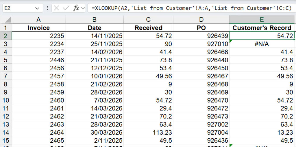
Example 1: Use XLOOKUP to Match Invoice Numbers in Excel

Scenario

A customer sends their paid‑invoices list. I want to bring the customer’s Amount Paid into Our List so I can compare it with what we received.

Formula (entered in cell E2, then copied down):

=XLOOKUP(A2,’List from Customer’!A:A,’List from Customer’!C:C)

Step‑by‑step

1. Click in the first cell where you want the customer’s amount to appear (E2 on Our List sheet).
2. Type = and start typing XLOOKUP(.
3. Select A2 (the invoice number in the current row) as the lookup value, followed by a comma.
4. Select column A, the Invoice Number column, on List from Customer as the lookup array, followed by a comma. Using the full column ensures that XLOOKUP can return values for new records without requiring a formula edit.
5. Select the Amount Paid column on List from Customer as the return array, followed by a closed bracket. Press Enter to confirm the formula.
   You now asked Excel to use the invoice number in A2 to find a match in column A of the List from the Customer sheet. Once it finds a match, return the dollar amount from column C on that sheet, in the same row.
6. Copy the formula down to return the customer’s amount for each invoice.

Where Excel finds a match, the amount from the customer’s list will be displayed. If a match isn’t found, the #N/A error will be shown.

Outcome

This places the customer’s amount beside your internal amount, allowing you to investigate further to identify what matches, what is different, and what is missing.

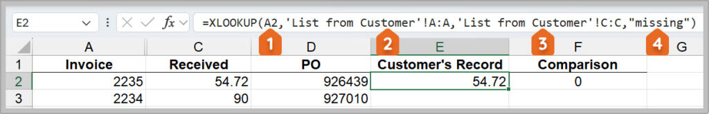
Example 2: Use XLOOKUP to Identify Missing Records in Excel

Scenario

If XLOOKUP cannot find a matching invoice number, it returns a #N/A error. Instead of showing #N/A, you can return a clear message by adding an additional argument to your XLOOKUP formula.

Formula:

=XLOOKUP(A2,’List from Customer’!A:A,’List from Customer’!C:C,“missing”)

Step‑by‑step

1. Click in the first cell of the Customer’s Record column (row 2).
2. Type = and start typing XLOOKUP(.
3. Select A2 as the lookup value, followed by a comma.
4. Select the Invoice Number column on List from Customer as the lookup array, followed by a comma.
5. Select the Amount Paid column on List from Customer as the return array, followed by a comma.
6. Add a fourth argument: “missing” and then type a closed bracket.

1. Press Enter to confirm the formula.
2. Copy the formula down the column.
3. Apply a filter to the column and select missing to see only unmatched invoices.

Outcome

Instead of messy #N/A errors, the worksheet clearly explains why the error appears, making reconciliation easier to understand and act on.

Stop and check: At this point, every invoice in Our List should have either a customer amount or a clear “missing” message. In the Customer’s Record column.

Example 3: Excel Comparison Formula to Check Whether the Amounts Match

Scenario

You’ve now identified missing records, but we now need to identify where records don’t match.

Formula:

You can add a simple check:

=IF(C2=E2,””,”check”)

Step‑by‑step

1. Click in the first empty cell where you want the Comparison to appear (row 2 of Our List).
2. Type =IF(C2=E2,””,”check”). If the amount in C2 equals E2, the cell will be left blank; otherwise, the word “check” will be entered into the cell.
3. Press Enter to confirm the formula.
4. Copy that formula down to quickly identify any invoices that need checking. Use a filter to quickly identify all records that need checking.

Outcome

You now have a simple cross‑check to confirm whether amounts match or require further attention.

Example 4: Excel Formula to Flag Underpayments and Overpayments

Scenario

If you’d like to go a step further, use the formula below to identify invoices that are short-paid or overpaid.

Tip: The formula looks long, but you don’t need to understand every piece to use it. Copy and paste the formula into Excel, then press Enter. After it works in the first row, copy it down the column.

Status formula (more difficult):

=IF(E2=”missing”,””,IF(C2=E2,””,IF(C2>E2,”over-paid”,”short‑paid”)))

Step‑by‑step

1. Insert a new column called Status.
2. Click in the first data cell of that column.
3. Enter the Status formula. This will help you determine whether the customer has overpaid or underpaid.
4. Press Enter.
5. Copy the formula down.

Tip: If you are working with a large list, apply a filter to the Comparison column to quickly identify records that need your attention, or filter the Status column to find where records where the customer has short‑paid or overpaid.

Outcome

Your reconciliation becomes a clear action list, allowing you to focus only on invoices that require follow‑up.

Example 5: Reverse XLOOKUP to Find Invoices Missing from Your List

Scenario

As a double‑check, compare the customer’s list back to your own.

Formula (entered on the customer sheet):

=XLOOKUP(A5,’Our List’!A:A,’Our List’!C:C,”missing from our list”)

This helps catch invoices that the customer has recorded that don’t appear in your report.

Step‑by‑step

1. Go to the List from Customer worksheet.
2. Click on cell E5 in the Our Amount column.
3. Type = and start typing XLOOKUP(
4. Select the customer’s Invoice Number as the lookup value, followed by a comma.
5. Select the Invoice column on Our List as the lookup array, followed by a comma.
6. Select the Received column on Our List as the return array, followed by a comma.
7. Add “missing from our list” as the if not found value, followed by a closed bracket.
8. Press Enter to confirm the formula.
9. Copy the formula down the column.
10. In cell F5, enter the comparison formula to identify the records to check
    =IF(C5=E5,””,”Check”)
11. Copy the formula down the column
12. Filter the columns to find records missing from our list or mismatched values.

Outcome

This reverse check highlights invoices the customer believes they’ve paid but don’t appear in your internal records — a critical final validation step. Our double-check confirms there is a $100 over payment on invoice 2464.  It also showed that the customer had possibly recorded the invoice number for invoice 2466 as 2646.

You will now have:

• One list with customer values pulled in beside your own.
• Clear labels showing what’s missing or different.
• The ability to filter both lists to identify only the invoices that need attention.

FAQs

Q. I’m getting #N/A, but the number looks exactly right. Why isn’t XLOOKUP finding a match in Excel?

A. This is one of the most common XLOOKUP issues I see, and it usually comes down to how the data is stored rather than the formula itself.

Check the following:

• The number might be stored as text. Even if it looks right, Excel treats text and numbers differently. A quick sign is that text often lines up on the left. To fix it, try: click the cell and use the warning icon (if shown), or use VALUE(), or multiply by 1 in a new column.
• There might be extra spaces. Spaces at the start or end of a cell will stop an exact match. To fix it, use TRIM() on the value, then use XLOOKUP on the cleaned result.

Q. Do both lists need to be sorted for XLOOKUP to work?

A. No. For exact matches (which is what you should use for reconciliations), XLOOKUP does not require sorted data. This is one of the big advantages over older lookup methods.

Q. Why is XLOOKUP returning the wrong result?

A. This usually happens when:

• The lookup value appears more than once in the lookup list
• The lookup array and return array are not the same size
• You’ve accidentally selected the wrong column as the return array

For reconciliations, always use a unique lookup value, such as an invoice or PO number.

Q. Can XLOOKUP return a value from a column to the left?

A. Yes — and this is one of the reasons it’s so popular. XLOOKUP can return values from any column, whether it’s to the left or right of the lookup column. You don’t need to rearrange your data.

Q. What happens if XLOOKUP finds more than one match?

A. XLOOKUP returns the first match it finds. By default, it will look from the top of the list to the bottom. If your lookup value isn’t unique, the result may not be the one you expect. That’s why checking for duplicates is such an important step before you start.

Q. Should I use full columns or fixed ranges in XLOOKUP?

A. For most everyday reconciliation work, using full columns keeps formulas simpler and more future‑proof, especially if new rows will be added later.

You might use a fixed range when:

• The data is static and will not grow
• You want to limit the lookup to a specific section
• You’re working with very large files and want to optimise performance
• There is unrelated data below the data you are looking up and you don’t want to include this in your results.

Q. Can I use XLOOKUP to return text, numbers, or dates?

A. Yes. XLOOKUP can return any data type — text, numbers, dates, or even blank cells — as long as the return array lines up with the lookup array.

Q. Do I still need VLOOKUP if I have XLOOKUP?

A. In modern versions of Excel, XLOOKUP can do everything VLOOKUP can — and more. I still teach VLOOKUP so you can understand existing spreadsheets, but for new work, XLOOKUP is the better choice.

Use this XLOOKUP checklist for your next reconciliation

• Do both lists share a unique ID (like an invoice number)?
• Is the lookup value stored as a real number (not text)?
• Are there any duplicates in the lookup column?
• Do you know which sheet is your “base list” (where results will appear)?

[Watch on YouTube] /  [Subscribe to our YouTube Channel]

Excel Practice File Download

Conclusion

Reconciling two lists doesn’t need to be manual or stressful.

With XLOOKUP, you can bring related records together, clearly see what’s missing or different, and focus only on the items that need action.

If you only remember one thing: start with a unique ID, use XLOOKUP to pull the records together, then compare.

Want to feel more confident with formulas?

Join my super-popular self-paced Excel course, ‘Excel 1-2-3, Go from Beginner to Pro,’ and learn how to use Copilot to save time and work smarter every day.

Or, book a live online coaching session with me to improve your skills and address any personal challenges.

If you’re not yet ready to take a course, I’m here to support you! Check out my YouTube tutorials and blog articles—they’re designed to help you build your skills and confidence. Let’s embark on your learning journey together!

YouTube: https://www.youtube.com/c/excelatwork
Search my Blog: https://www.excelatwork.co.nz/blog/