Once you know how to enter data into an Excel worksheet, you will be setting up tables of data quickly.
When you haven’t been shown how to enter data, it can be a little tricky, so follow the steps below to learn tips and tricks for entering your data easily into your worksheet.
Entering data into an Excel worksheet
You can enter either values (numbers and dates) or labels (text) into any cell within the worksheet.
1. Move the cell pointer to the required cell and type the data. While you type the data, you will notice that it appears in both the worksheet (in the example below, the text appears in cell A1) and in the Formula Bar.

2. Press ENTER to enter the information into the cell. Your cell pointer will move down to the cell below.
Tip: If you press the ESC key instead of ENTER the data will not be entered into the cell.
Deleting and replacing data
- To delete data, select the cell containing the data and then press DELETE.
- To replace data, just type directly over the top of the existing cell contents. The new data will replace the old.
Using Undo and Redo
There will be times when you enter data only to realise you have made a mess of things.
Most times, you want to go back to where you were before the mistake was made. If this happens, you can click the fabulous “Undo” button, which will undo the last thing you did.

You can keep clicking it until you get back to a point where you feel in control again.
If you go too far back, you can click the Redo button to move forward a step again. These buttons are fabulous, and you use them a lot.
Overlapping data
If you enter data that does not fit the column width, it will overlap into the next column. In the example below, the text ‘Travel Expenses’ is entered into cell A1; however, it looks as though the text is included in cell B1. With cell A1 selected, we can see in the Formula bar that both words are indeed in A1.

If you are not using the column in which the text overlaps, you may leave it as it is. However, as soon as you place text into a cell that has been overlapped, it will look as if your text has been lost. In the example below, the text ‘Amount ex GST’ has been entered into cell C3. However, the content of cell D3 is hiding part of the content of C3.

By selecting C3, the entire cell’s content can be seen in the Formula Bar. However, to view the entire contents of cell C3, the width of column C needs to be adjusted.
Working with columns
The standard column width for Excel is 8.43 character spaces. You can change the column width by dragging with your mouse on the column headers or by double-clicking between two column headers.
Tip: If multiple columns require the same width, select the columns and widen one of them with the mouse. The rest will be adjusted to the same width.
Adjusting the column width
To use your mouse to adjust the column width:
1. Move your mouse pointer over the column’s right edge in the column header area. Your mouse pointer should change to a double-headed arrow.

2. Click and drag to the right to expand or to the left to shrink the column width to the required size.

You will now be able to see your entire text. Continue dragging until all columns are the width you require.

Tips: To quickly adjust the column width to fit the widest entry, move your mouse pointer over the lines between the column headers. When the pointer becomes a double-headed arrow, double-click.
Use the same method for adjusting the height of any row. Just move the mouse pointer over the line separating the rows. When the pointer becomes a double-headed arrow, drag or double-click to adjust the row height or double-click to set the height to fit the tallest entry.

By the way, row heights will automatically alter if the font size of the data is altered.
Extra info: To set a column width to a precise measurement, on the Home tab in the Cells group, select Format and then select Column Width. Type the desired width in the Column Width box, and then click OK to accept the new column width.
What do hash signs mean in Excel?
If you ever see a cell containing ######## (hash signs), it means the column isn’t wide enough to display the content. Just extend the width, and the content will become visible.
Making changes to the data
Once you have entered data into your worksheet, you can edit the data in a number of ways.
- Select the cell and then click on the Formula bar. A flashing insertion point will be placed into the bar. Use the arrow keys on the keyboard to move the insertion point. Make the changes you require, and then press ENTER.
- You may also type directly over the data in the cell with new data and press ENTER. The new data will replace the old.
- Double-clicking a cell or pressing F2 lets you edit its contents directly on the worksheet. Make the changes and then press ENTER to update the cell.
AutoComplete
AutoComplete allows Excel to automatically complete an entry for you.For example, if you have typed text in the cells above, as soon as you start typing a letter or two in a cell below, Excel will check the list above for a matching entry and complete the entry for you.
 This can be very useful when you must make the same entry several times.
To accept the entry, press ENTER. To reject the displayed entry and type something different, either ignore it and type right over it or press DELETE.
Was this blog helpful? Let me know in the comments below.
Want to Learn Excel Properly?
Join the Excel at Work Learning Hub
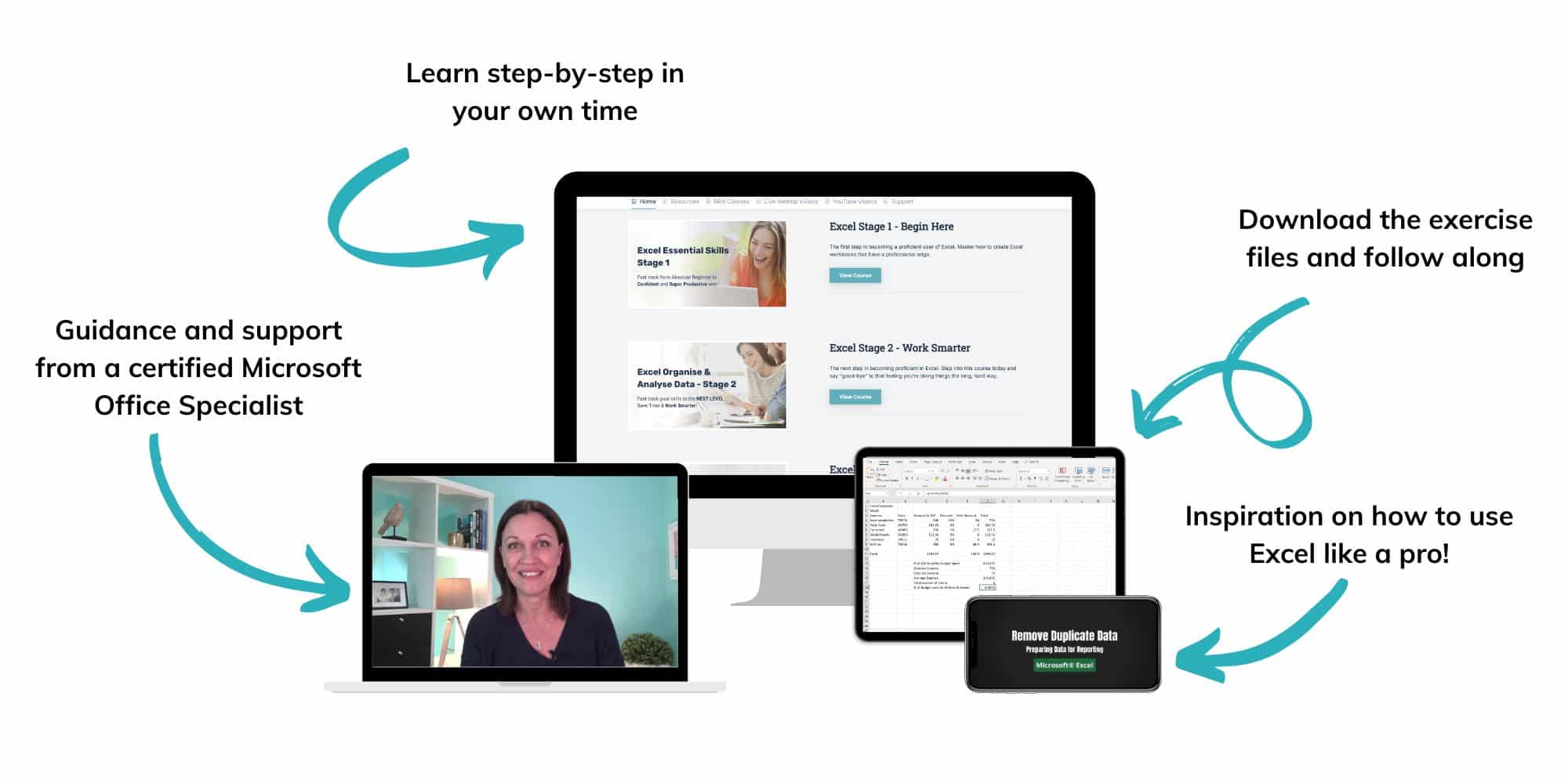
The Excel at Work Learning Hub is an online self-paced Excel training membership designed for people who use Excel at work—in offices, on sites, in schools, in small businesses, and everywhere in between.
Go from Beginner to Confident – Guaranteed!
Only $59NZ /month
Cancel anytime • No pressure • 14-day 100% Money Back Guarantee

Certified Microsoft Office Specialist
Was this blog helpful? I’m here to empower your journey with Excel, aiming to make your daily tasks more efficient and boost your potential.
Share your thoughts in the Comments below – your insights not only enrich others, they also help me tailor future content to your needs.
And if you’re looking to take a step further, join our exclusive ‘Insider Group‘. As a member, you’ll receive Weekly Super-Tips, and early access to in-depth tutorials. Sign up Today!
Happy Excel-ling!!


It kind of complicating but, gives alot of information
Thanks Luciana. I hope you found it helpful.