Use TRIM with SUBSTITUTE Function in Excel to Remove Spaces the TRIM Function Misses

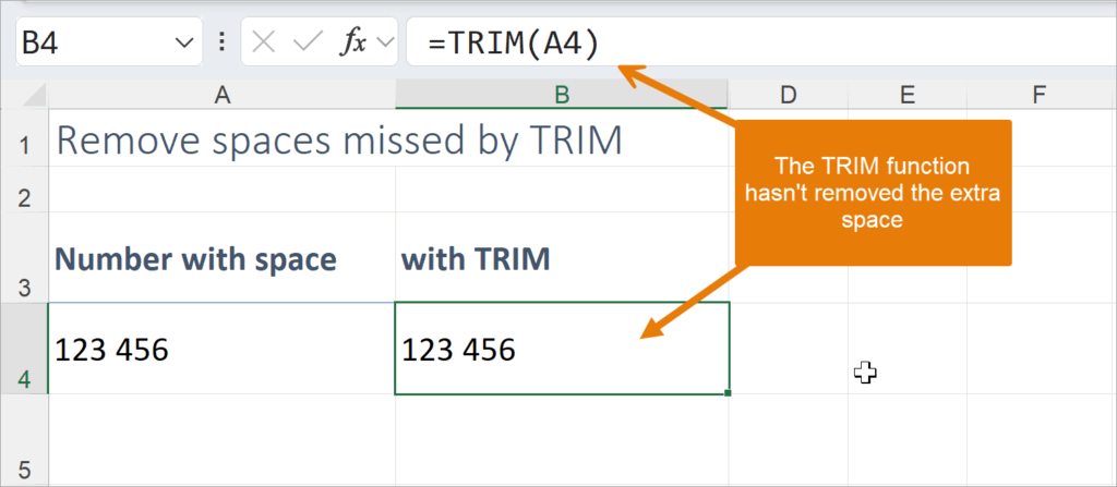
Have you ever used the TRIM function in Excel, only to find that it didn’t remove all the spaces and isn’t working as expected?

So, why doesn’t TRIM remove all spaces in Excel? If Excel’s TRIM function isn’t removing spaces, it’s likely dealing with hard spaces, also called non-breaking spaces.

Because TRIM only removes regular spaces. If your data contains hard spaces, TRIM won’t recognise them.

You can fix this using SUBSTITUTE to replace those hard spaces with regular ones, and then use TRIM to clean the rest. This combo helps you remove even the spaces TRIM normally misses.

In this post, I’ll show you two easy ways to remove spaces that the TRIM function misses, along with a bonus tip on how to clean up even the most stubborn spacing issues.

Excel Practice Files

What’s The Difference Between Regular And Hard Spaces In Excel?

• A regular space (what the TRIM function can remove). Excel refers to this type of space using the character code CHAR(32).
• A non-breaking space (which TRIM ignores) is character code CHAR(160).

You usually don’t notice the difference just by looking at the cell, but Excel treats them as entirely different characters.

How Do Non-Breaking Spaces Get Into Excel?

They often sneak in when you:

• Copy and paste from a website, PDF, or HTML-based system
• Export data from accounting software, CRMs, or browser-based apps
• Import values from third-party tools or emails

If TRIM isn’t cleaning your cells properly, a hard space is likely the culprit.

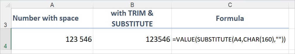
Fix #1: Use SUBSTITUTE With VALUE To Remove Spaces In Numbers

Sometimes a number in Excel isn’t really a number — it’s text pretending to be one.

This often happens when a space sneaks into the cell. Even a single space between digits will cause Excel to treat the value as text, regardless of whether the space is a regular one (CHAR(32)) or a non-breaking space (CHAR(160)).

And while the TRIM function can remove extra spaces at the beginning, end, or multiple spaces between words, it won’t remove a single space between numbers, which is often the issue when cleaning imported or copied data.

In the example below A4 contains the number 123 456 (with a space in the middle). Excel won’t treat this as a number, and formulas like =SUM() or =COUNT() won’t work properly.

The Solution:

• Use a combination of the SUBSTITUTE and VALUE functions to:
• Replace any space with nothing (“”).
• Convert the result into a proper numeric value that Excel will recognise.

The Formulas:

To remove regular spaces (CHAR(32)):
=VALUE(SUBSTITUTE(A4,CHAR(32),””))

To remove non-breaking spaces (CHAR(160)):
=VALUE(SUBSTITUTE(A4,CHAR(160),””))

To remove both types of spaces:
=VALUE(SUBSTITUTE(SUBSTITUTE(A4,CHAR(160),””),CHAR(32),””))

What It Does

• SUBSTITUTE(A4,CHAR(…),””) replaces the regular or non-breaking space with nothing, removing it completely.
• VALUE(…) converts the cleaned text into a real number that Excel can calculate with — no more formula issues or weird results!

Steps To Clean Hard Spaces From A Number Using SUBSTITUTE And VALUE:

1. Click into a blank helper cell next to the number with the issue (e.g., if the messy number is in A4, click into B4).
2. Type the formula, e.g. =VALUE(SUBSTITUTE(A4,CHAR(160),””))
3. Press Enter — the result will now appear as a proper number.
4. (Optional) Copy and paste the cleaned value over the original using Paste Values.
5. Double-check by using SUM or COUNT on the new value — Excel should now treat it like a number (not text)

Fix #2: Remove Spaces The TRIM Function Misses In Excel

The TRIM function in Excel is excellent for cleaning up unwanted spaces — but it only removes regular spaces (CHAR(32)).

If your data includes non-breaking spaces, with character code CHAR(160)), TRIM won’t touch them.

The Solution:

That’s where the SUBSTITUTE function comes in.

By using SUBSTITUTE first to replace the hard spaces with regular ones, you allow TRIM to then do its job and clean up any remaining extra spaces.

Use This Formula:

=TRIM(SUBSTITUTE(A4,CHAR(160),CHAR(32)))

What It Does:

• SUBSTITUTE(A4,CHAR(160),CHAR(32)) searches the cell for hard spaces and replaces them with normal spaces.
• TRIM(…) then removes any extra spaces between words, clears leading and trailing spaces and leaves you with a clean, readable result

Steps To Remove Spaces The TRIM Function Misses Using SUBSTITUTE And TRIM

1. Click into a blank helper cell next to the cell with the space issue (e.g., if the messy text is in A7, click into B7).
2. Enter this formula: =TRIM(SUBSTITUTE(A7,CHAR(160),CHAR(32)))
3. Press Enter — the cell will return a cleaned version of the text.
4. Check that the extra spaces are gone — leading, trailing, and multiple spaces between words should be removed.
5. (Optional) If needed, copy the result and paste it as values to replace the original data.

BONUS TIP: How Do You Extract Clean Text From A Cell With Too Many Spaces?

Sometimes a cell contains valuable information — such as a name followed by an email address — but it’s cluttered with far too many spaces, making it difficult to separate the two parts cleanly.

In the example below, cell A4 contains the person’s name and email address, separated by multiple spaces.

Solution:

The TEXTBEFORE and TEXTAFTER functions, combined with the TRIM function, will help you remove spaces and extract the necessary data from the cell.

Formula To Extract Text Before Spaces

Use TEXTBEFORE to extract all the text before the second space, which gives you the first and last name.

= =TEXTBEFORE(A4,” “,2)

What It Does:

• It reads the cell from left to right and finds the second space. In the example above, the second space comes after the surname “Brown”.
• Then it returns everything before that second space, which is the first and last name.

It doesn’t matter how many spaces are between the name and the email — the function stops right at the second space it finds and cleanly returns the first and last names.

Steps To Extract Text Before Spaces

1. Click into a blank helper cell next to the messy data (e.g., if the full text is in A4, click into B4).
2. Enter this formula: =TEXTBEFORE(A4,” “,2). Note, there is one space between the quote marks.
3. Press Enter — Excel will return the first and last name. Excel looks for the second space in the cell and returns everything before it — even if there are lots of spaces after the name.

Formula To Extract Text After Spaces

=TEXTAFTER(TRIM(A5),” “,2)

What It Does:

• TRIM(A5) removes all the extra spaces, leaving one space between each word or value.
• TEXTAFTER(…,” “,2) skips the first two “chunks” of text (in this case, the first and last names) and returns everything after the second space, which is the email address.

Steps to Extract Text After Spaces

1. Click into another blank helper cell, such as B4.
2. Enter this formula: =TEXTAFTER(TRIM(A5),” “,2). Note, there is one space between the quote marks.
3. Press Enter — Excel uses the TRIM function to remove all the extra spaces, and then the TEXTAFTER(…,” “,2) formula skips the first two words (first and last name) and returns everything after, which is the email address.

Super Tip!

You can use the TEXTBEFORE and TEXTAFTER functions to get content from the right side of a cell by using a negative number, for instance. This formula, =TEXTAFTER(A6, ” “, -1), is another way to extract the email address after the last space in cell A6.

Conclusion: How To Remove Extra Spaces In Excel When TRIM Doesn’t Work

Unwanted spaces in Excel can cause formulas to break, data to look messy, and calculations to fail — especially when TRIM isn’t enough on its own.

Now that you know how to remove extra spaces, including non-breaking (hard) spaces that TRIM misses, you’ll be able to clean up numbers, names, email addresses, and more with confidence.

Whether you use SUBSTITUTE, TRIM, VALUE, or the powerful TEXTBEFORE and TEXTAFTER functions, each method offers a practical solution for a different scenario — no matter how messy your data is.

A cleanup goes a long way — and now you’ve got the tools to handle it!