How to Copy Cell formats to other cells in Excel

Do you spend hours perfecting the format of a single cell in Excel, only to realise that you need the same formatting applied to numerous cells or a larger range?

If done manually, this can be a tedious and time-consuming task. Fortunately, the powerful Format Painter in Excel provides a solution. It works like a digital paintbrush, enabling you to effortlessly copy formatting from one cell to another with just a few clicks.

Assume you have a spreadsheet with a table that contains different product groups, current prices, and cells that calculate the price increases for each group. To draw attention, you want to highlight the product group headings and the cell showing the percentage increase. Instead of manually formatting each cell, you can use Format Painter to copy the formatting from one cell to another quickly.

It’s like having a magic wand that instantly transforms your data into a visually appealing and consistent format.

In the upcoming sections, we’ll dive deep into the Format Painter feature and how it can help you in many ways. You’ll be able to copy formatting to multiple cells and use it with conditional formatting.

With the Format Painter, you can save time and make your Excel spreadsheets look professional and stylish. This tool is an asset that will help you take your Excel skills to the next level.

1. Where is the Format Painter in Excel

The Format Painter feature in Excel is a great time-saver. It allows you to quickly apply the same formatting, including font styles, cell borders, and fill colours, to multiple cells or ranges without manually formatting each one.

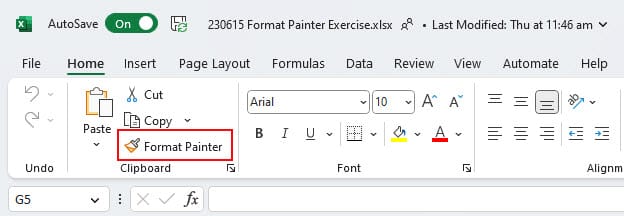
Head to the Home tab on the Excel Ribbon to access the Format Painter tool. You can find it in either the Clipboard or Clipboard/Clipboard group section. Look for the paintbrush icon representing the tool and click on it to activate it.

2. Copy Cell formats to other cells

1. To copy the desired formatting to another cell, select the cell that already has the formatting you want to use as a reference. This source cell will be the basis for the formatting you plan to copy. In the example below, we will select cell C4, which has the formatting we want to copy.

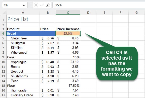
2. From the Home tab in the Clipboard group, click the Format Painter button.

3. When you activate the Format Painter tool, the mouse pointer changes into a paintbrush icon. This signifies that the tool is ready to copy formatting from the source cell.

4. To apply the formatting, go to the target cell. Click on the cell where you want to apply the formatting, and it will automatically adopt the formatting of the source cell. In this example, we selected cell C9.

5. Once you release your mouse, the formatting will be applied.

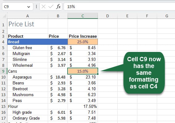
6. Once the formatting has been applied to the target cell, the tool is automatically turned off (deactivated). This indicates that the formatting from the source cell has been successfully copied and applied to the desired destination cell.

3. Copy formatting in Excel to Multiple Cells

Using the Format Painter to copy formatting to multiple cells at once can significantly save time and effort when working with large Excel data sets.

In the example below, we want to continue copying the heading and input cell formats to additional product group headings in our data set.

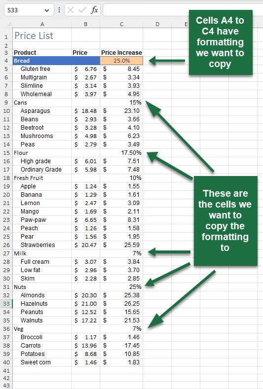
1. To apply formatting to other cells, first select the cells with the desired formatting. These cells will act as the source from which the formatting will be copied. In the following example, we copy the format from cells A4 to C4.

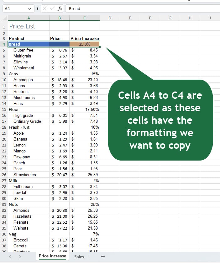
2. From the Home tab in the Clipboard group, double-click the Format Painter button.

3. When you activate the Format Painter tool, the mouse pointer transforms into a paintbrush icon – a sign that the tool is ready to copy the formatting from the source cell.

4. To apply formatting, click and drag your mouse to select the cells or ranges you want to modify. Then, drag your cursor across the ranges of cells. In the example below, we copied the formatting to cells A9 to C9.

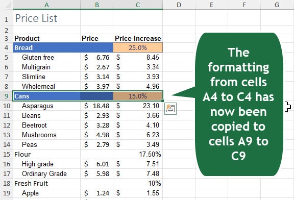
5. After selecting the desired cells or ranges, continue to another set of cells that require formatting and select these cells. Repeat until all cells are formatted as required.

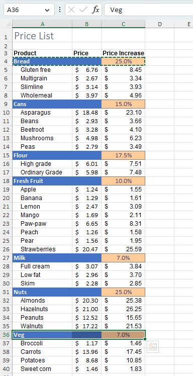
6. To turn off the Format Painter, press the ESC key or click the Format Painter button again.

By following these steps, you can efficiently use the Format Painter to copy and apply formatting to multiple cells in Excel. This feature saves time and effort, especially when maintaining a consistent appearance across different spreadsheet sections.

4. How to Copy Conditional Formatting in Excel

Excel’s Conditional Formatting is a robust tool that automatically formats cells based on specific conditions or criteria. 

Let’s say you have a sales data spreadsheet with a column containing the total sales value for each sale. You want to highlight the cells that meet a certain value threshold in a specific colour to draw attention. Conditional Formatting can help you achieve this.

To optimise Conditional Formatting, you can combine it with the Format Painter tool, which efficiently applies and extends conditional formatting across multiple cells or ranges. 

Follow this detailed step-by-step guide to learn how to use the Format Painter with Conditional Formatting.

How to create a Conditional Formatting Rule in Excel

First, create a conditional formatting rule. In the example below, we will highlight any sales that are greater than $4,700:

1. Select the range of cells containing the sales data.

2. Go to the Home tab in the Excel Ribbon and click on Conditional Formatting.

3. From the drop-down menu, choose Highlight Cells Rules and then Greater Than.

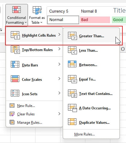
4. In the dialogue box that appears, enter the threshold value that determines what constitutes a high sale. In our example, this will be $4,700.

5. By default, the cells with sales higher than the threshold will be formatted with ‘Light Red Fill with Dark Red Text’.

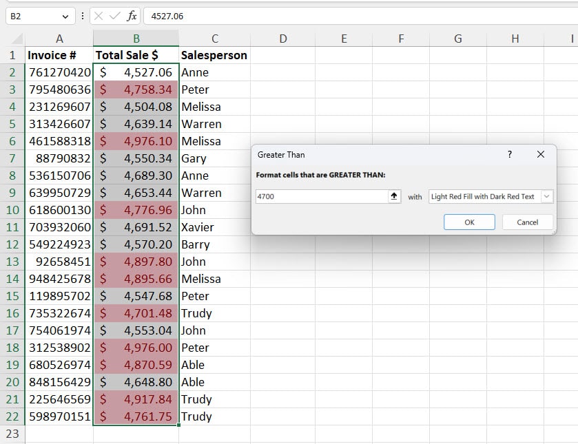
6. To select a different formatting style to apply to the cells with sales higher than the threshold, click the drop-down arrow on the Format box to select a pre-set format or create a Custom format. A Custom format could be a specific font colour, cell fill colour, or other formatting option.

7. Click OK to apply the Conditional Formatting.

After applying the Conditional Formatting, any cells in the selected range with sales higher than the specified threshold value of $4,700 will be automatically highlighted according to the chosen formatting style. This allows you to quickly identify and analyse the cells with the highest sales values in your spreadsheet.

Copying Conditional Formatting Rules in Excel

If you enter new data outside the range formatted with the Conditional Formatting rule, use the Format Painter to paint the rule over the new data. In the example below, new data has been entered into rows 23 to 26.

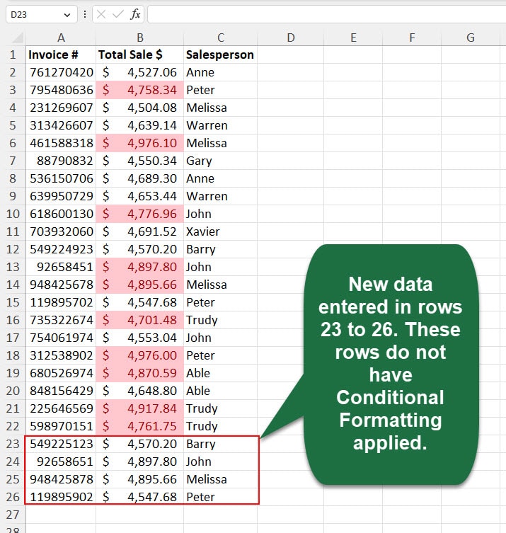
1. Select a cell with the Conditional Formatting applied. In the example below, we selected cell B2, but any cell with the Conditional Formatting applied could be selected.

2. From the Home tab, click the Format Painter button. The mouse pointer will now change to a paintbrush.

3. Select the range of cells where you want to apply the same Conditional Formatting. You can click and drag to select multiple cells or click on individual cells while holding the left mouse button. 

4. Excel will apply the Conditional Formatting rule from the original cell to the selected range of cells, extending the formatting to the new data.

5. Using the Format Painter, you can easily extend the Conditional Formatting rule to new data without manually setting it up again. In the example below, we selected cells B23 to B26, the newly pasted cells with no conditional formatting applied.

Following these steps, you can effectively harness the Format Painter with Conditional Formatting in Excel. This combination allows you to create complex formatting rules based on specific conditions and effortlessly apply them to different cells or ranges, saving time and ensuring consistent formatting throughout your spreadsheet.

Watch the Excel Copy Cell Formats Tutorial

[Watch on YouTube] / [Subscribe to our YouTube Channel]

Conclusion on the Format Painter in Excel

Excel’s Format Painter is a highly flexible tool that can help you save time and maintain consistency in formatting. It allows you to effortlessly transfer formatting styles from one cell to another, ensuring a professional-looking spreadsheet. Don’t be afraid to experiment with the Format Painter to improve your Excel skills and increase productivity. Take advantage of this powerful feature and unlock its full potential in your Excel workflow.

Was this blog helpful? I’m here to empower your journey with Excel, aiming to make your daily tasks more efficient and boost your potential.