How to Remove Blank Rows in Excel

Needing help to remove blank rows in Excel?

Let’s look at several options as each one is super useful depending on the number of blank rows you need to remove.

1. How to remove a blank row in Excel

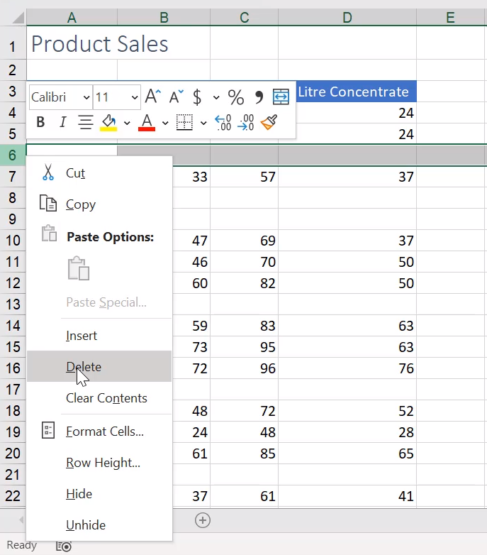
1. To remove a single blank row, right click over the row number. For example, if you wanted to removed row 6, right-click on top of the number 6 in the row header area. This will select the entire row and display the shortcut menu.

2. Select Delete from the shortcut menu. The row will be removed.

2. How to remove blank rows in Excel

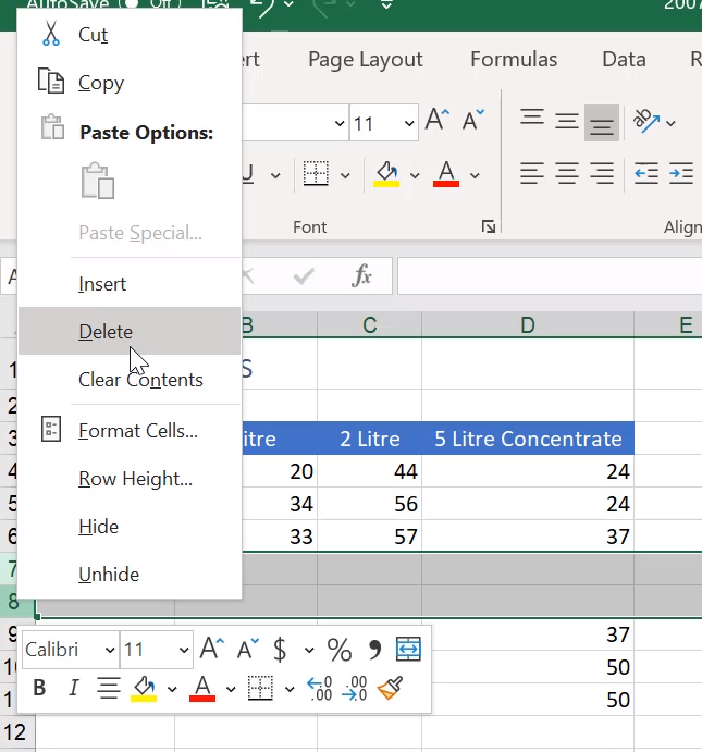
To remove adjacent blank rows, click and drag over the row numbers to select the blank rows, right click any of the selected row numbers, and then click Delete.

To remove non-adjacent blank rows…

1. Click the row number of the first blank row you want to remove. This will select the entire blank row.

2. Press and hold down the Ctrl key and then click the row numbers of the additional blank rows you want to remove. In the example below, row 10 was first selected and then rows 14 and 18 have been added to the selection using Ctrl + click.

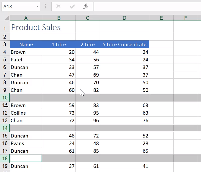
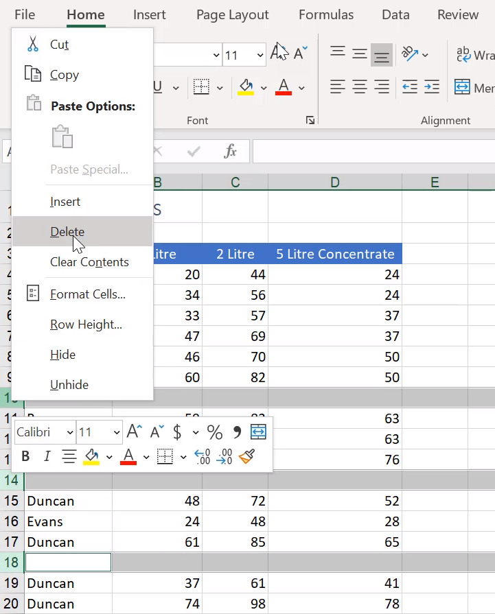
3. Now right click any of the selected row numbers and then select Delete from the shortcut menu. All of the selected blank rows will be removed.

3. Shortcuts to remove blank rows in Excel

1. First click on to any cell in the blank row.

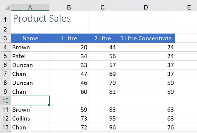
2. Then, press Shift + Spacebar to select the entire row.

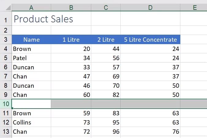
3. Once the row is selected, can press Ctrl + – (minus sign) to delete the row.

4. Filter to remove blank rows from a large list of data

Using your Ctrl + right click to select and remove random blank rows is good when you have a small list of data. However, when you have a large table of data with a large number of empty rows this isn’t the quickest way to delete them.

Use Filter to quickly remove blank rows in an Excel list.

Filter to find blank rows in Excel

1. Select all the data in your list, including the empty rows.

Hint: To quickly select from the top to the bottom of a large list, including the blank rows, first select the top left cell in the list. Pres and hold the Shift key and then click the bottom right cell of the list. This will select all cells in between both points.

Using this point-to-point click is better than using Ctrl + A to select the data, because Ctrl + A will only select the first empty row. You want to include the entire list, including the empty rows. Therefore, a point-to-point selection makes selecting a better option.

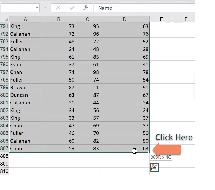
2. Scroll back up the screen to the top of the list so that you can see the headings at the top of each column.

3. Go to the Data tab and then select Filter. This will turn on Filter.

4. Now go to any of your column titles at the top of your list and select one of the Filter drop-down arrows (as shown below).

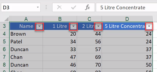
5. Remove the check mark from the Select All option in the list and then scroll right to the bottom of the list. Select (Blanks).

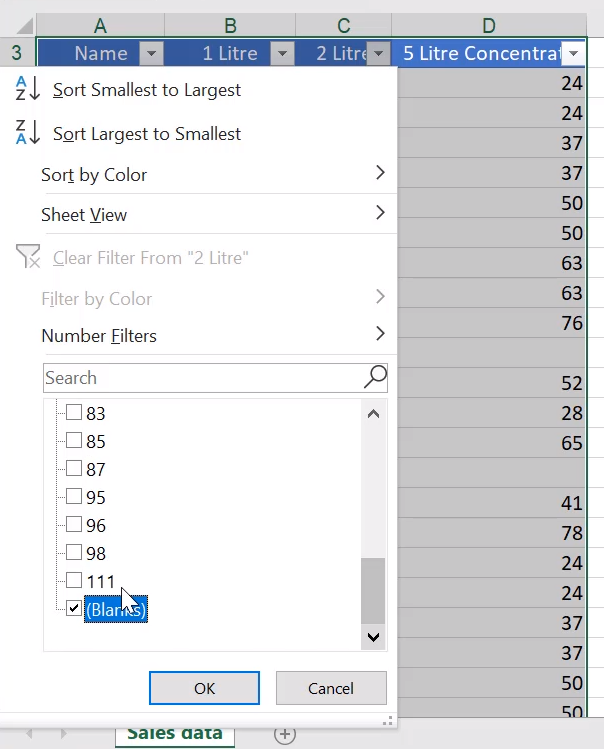
6. Click OK.

Remove blank rows from the filtered data

Excel will filter and display only the blank rows. A blue row number indicates that each of the rows is part of the filtered data set.

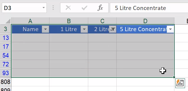
7. Now select all the rows with blue numbers. Be sure to select the entire row. The best way to select the entire row is to click and drag over the row numbers. 

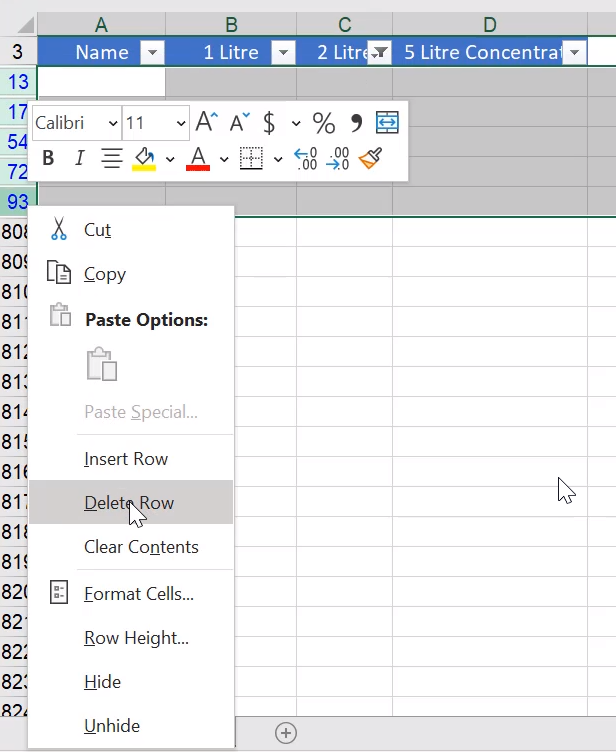
8. Right-click over the row numbers and then select Delete from the shortcut menu.

9. On the Data tab, click the Clear button to remove the Filter. 

10. You will now see all of your data with the blank rows now removed.

5. Remove blank rows in Excel using Go To Special

If you’re not familiar with filtering try this…

1. Select the entire list of data and then press Ctrl + . (period or full-stop) to quickly move back to the top of the selected data.

2. Select the Home tab and then click Find & Select. Now, click Go to Special.

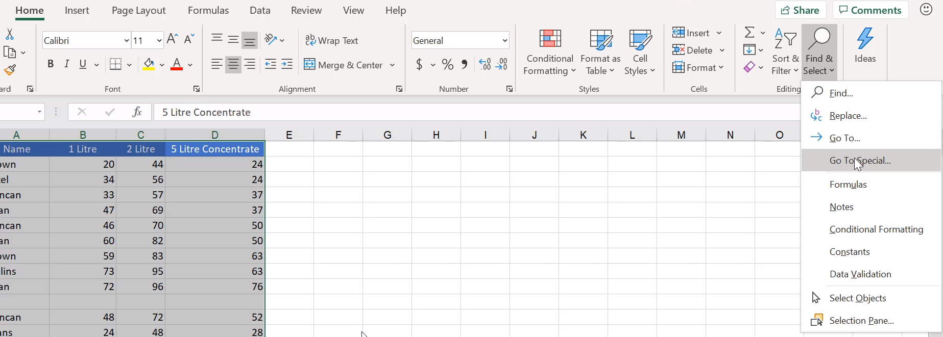
3. Select Blanks in the Go To Special dialogue box. This option tells Excel to only select blank rows or blank cells.

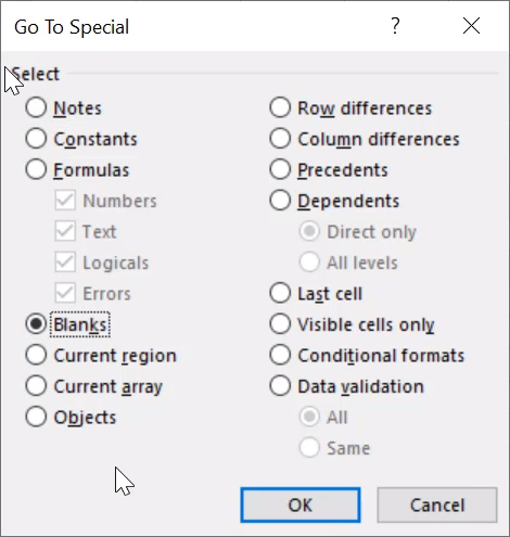
4. Click OK. This will selected all the blank rows.

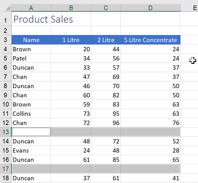
5. Press Ctrl + – and the Delete dialogue box will appear asking you what you want to do.

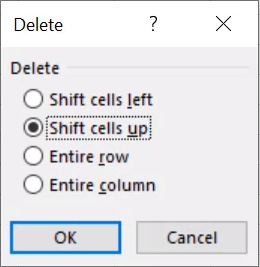
6. Select Entire row and then click OK.

The blank rows will now be removed.

Useful tip: Ctrl + Down Arrow will take you to the first instance of an empty row. So, if you press this you will be able to see if there are remaining rows in your data table that haven’t been removed.

6. Remove blank rows at bottom of Excel worksheet

If you are trying to remove ALL the blank rows at the bottom of your data you may have found that the options above haven’t helped, and the blank rows still remain.

This is because Excel has a set number of rows per worksheet. These will remain visible, even if you try to delete them.

However, you can hide them.

1. Click on a cell in the first row that you want to hide.

2. Now press Shift + spacebar. This will select the entire row.

3. Now press Shift + Ctrl + Down Arrow. This will select to the very last row in the worksheet.

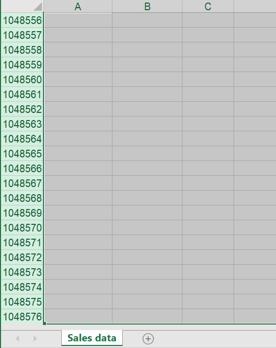
4. Place your mouse pointer over the row numbers and right-click. Select Hide from the shortcut menu.

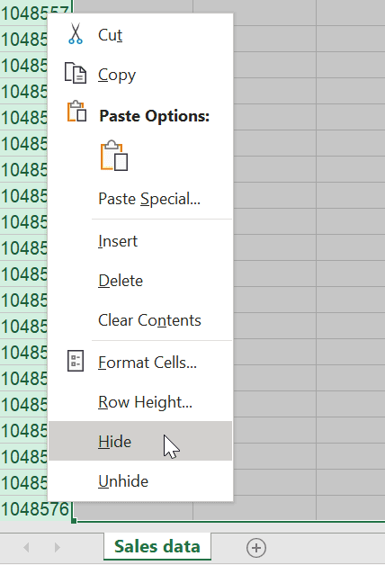
The rows will now be hidden. The rows will remain in the worksheet but will not be visible.

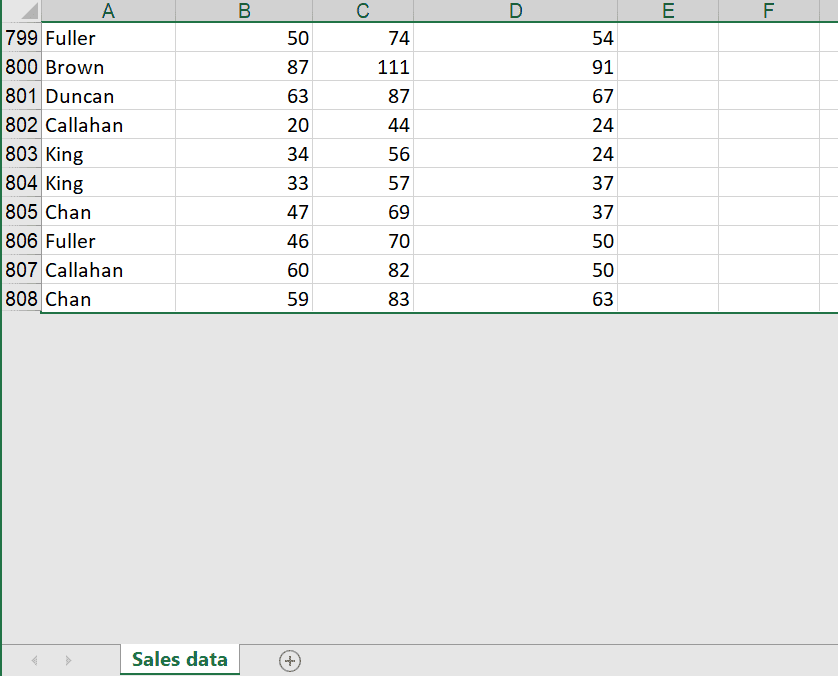
7. How to unhide only rows at the end of worksheet

Hiding the empty rows is quite easy. However, bringing them back can be a little fiddly.

If you only have hidden rows at the end of your data, you can easily select the entire worksheet (press Ctrl+ A until the entire worksheet is selected) then right-click over the row numbers and select Unhide from the shortcut menu.

However, if you have hidden rows inside your data area the above option will unhide these as well.

To unhide only rows at the end of the worksheet follow the steps below…

1. Press F5 to open the Go To dialogue box. In the Reference box type A1048576 and then click OK.

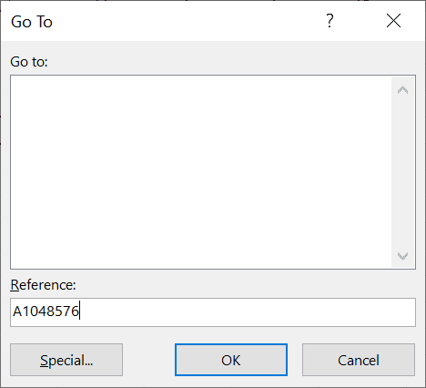
2. This will move the cell selector to the last row in column A. You still won’t be able to see the cell on screen at this point. To see the row, from the Home tab select Format, Hide & Unhide, Unhide Rows.

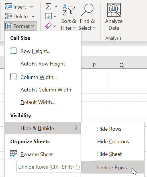
3. The last row will now be visible below the last row of your data.

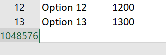
4. Now select over the last row of your data and row 1048576 so that both rows are selected. In doing this you are showing Excel that you want to unhide any hidden rows that are between the two selected rows.

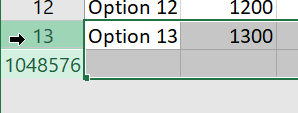
5. Right-click over either of the row numbers so that the shortcut menu is shown, and then select Unhide.

Your hidden rows will once again be visible.

Watch the Excel how to remove blank rows Tutorial

[Watch on YouTube] / [Subscribe to our YouTube Channel]

Was this Blog helpful? Let me know in the comments below.