How to Create Drop Down Menu in Excel (Drop Down List)

Learn how to create a drop-down list in Excel.

In this blog you will learn two different ways to create a drop-down list and the advantages of each as well as an extra step needed for older versions of Excel when creating a drop-down list from another worksheet.

Let us look at an example in Excel.

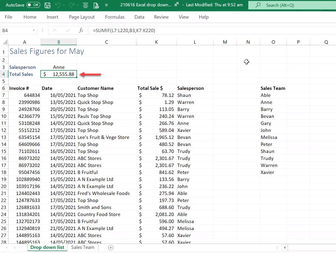
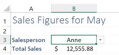
A SUMIF function is in cell B4, giving the total of sales made by Anne.

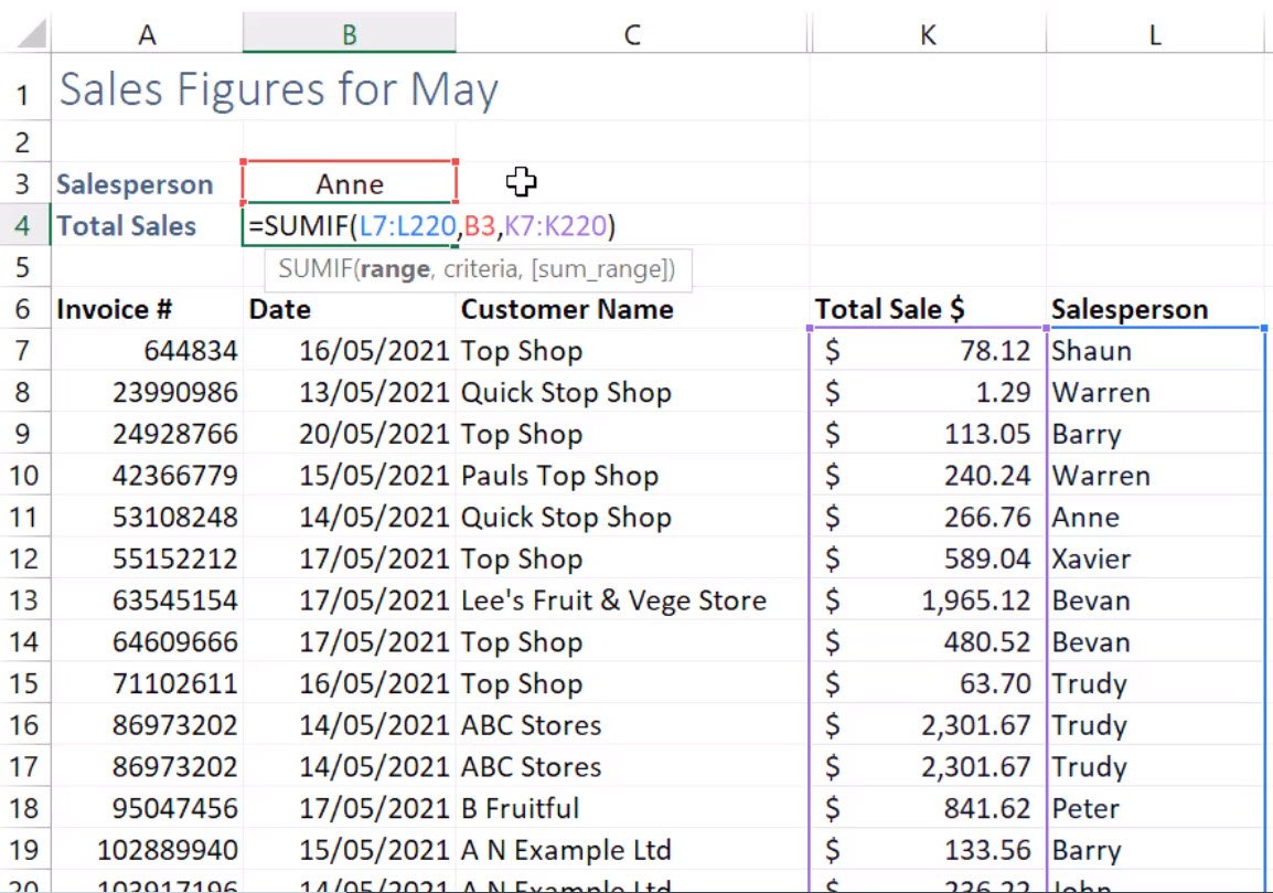
Note: The SUMIF function in B4 is looking at Anne’s name in cell B3 and bringing back her total sales from the ‘Total Sales $’ column.

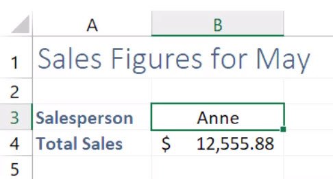
Wouldn’t it be nice to have a drop-down option on cell B3 where you could select any member of the sales team and have their total sales be pulled through into cell B4? The following steps will show you how to achieve this.

Option #1 – Create a Drop Down List from the Same Worksheet

Start with a pre-existing list on your worksheet.

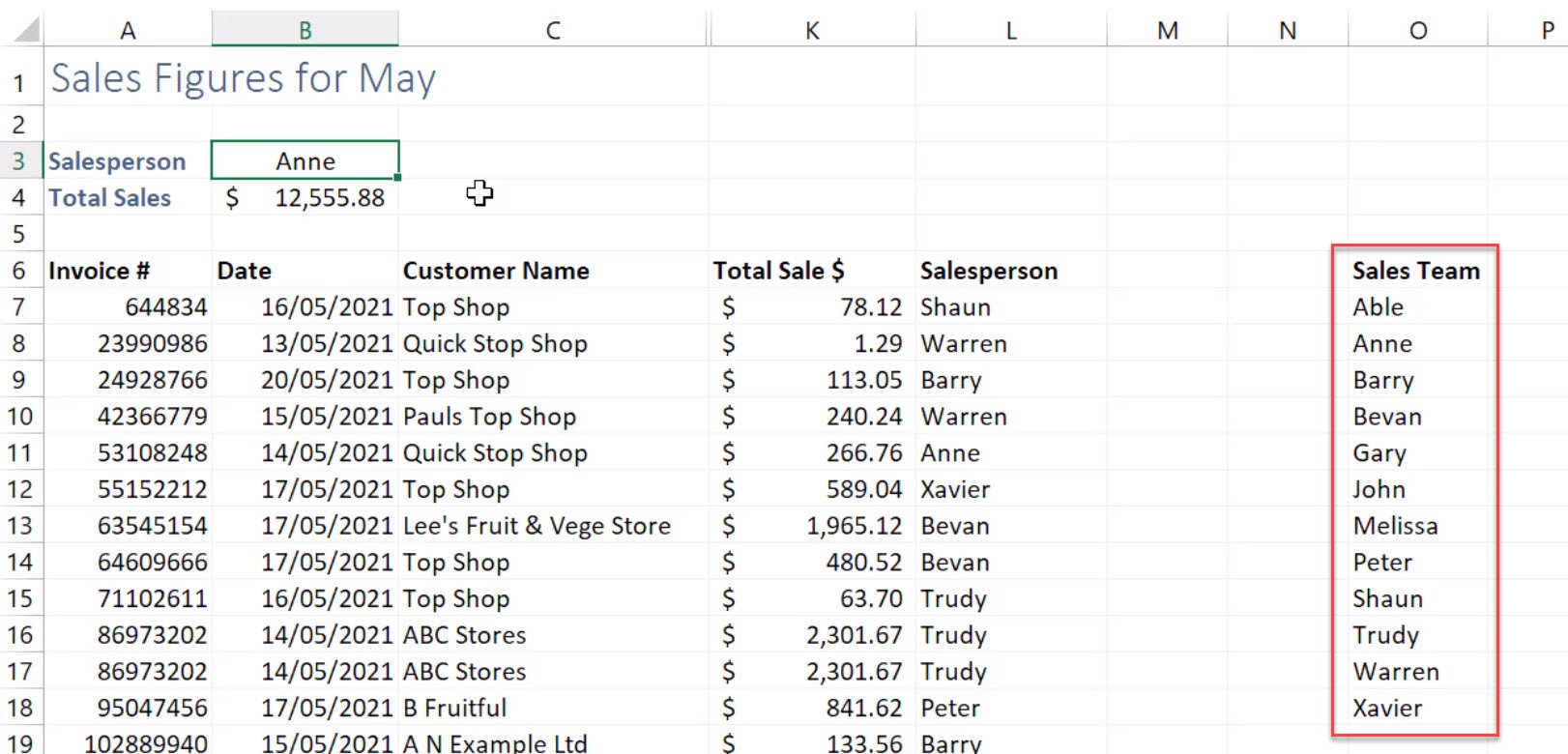
Tip: a good idea is to sort your list in a logical order before creating your drop-down list. In this example, the list is ordered alphabetically.

Click on the cell you want the drop-down list on. For this example, we want the drop down information in cell B3.

Go to the Data tab and select Data Validation.

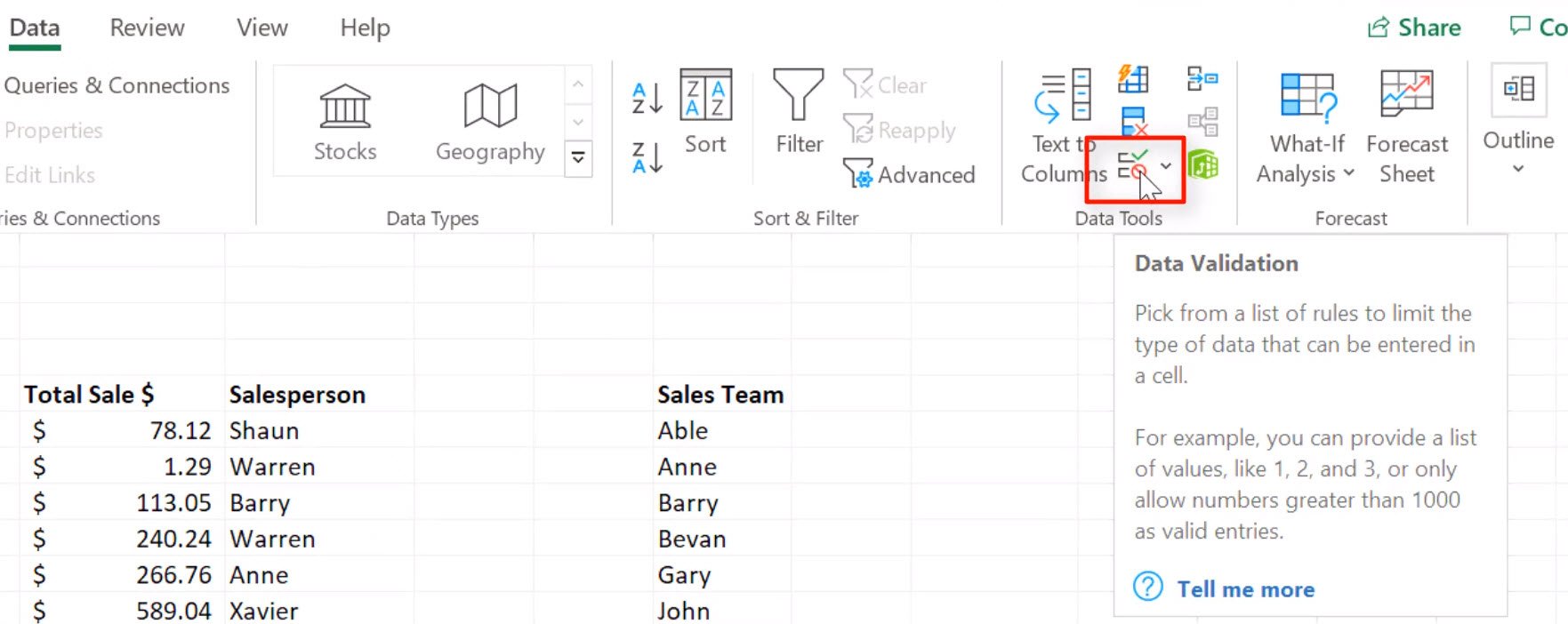
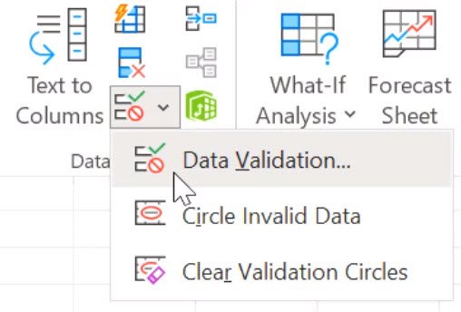
Note: You can also select Data Validation by selecting the drop-down arrow then selecting Data Validation.

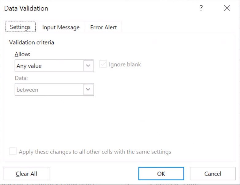
The Data Validation dialog box will appear.

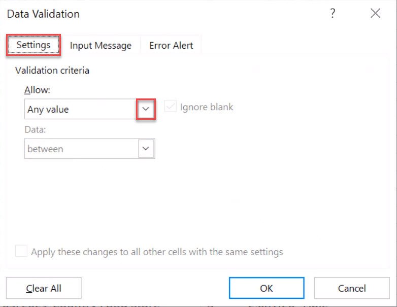
On the Settings tab, select the drop-down arrow underneath Allow.

Select List.

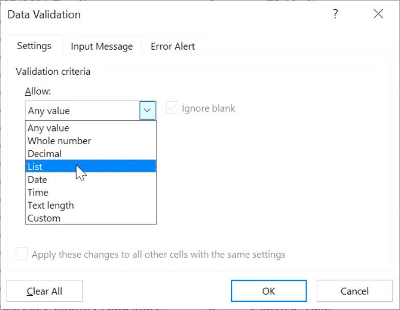
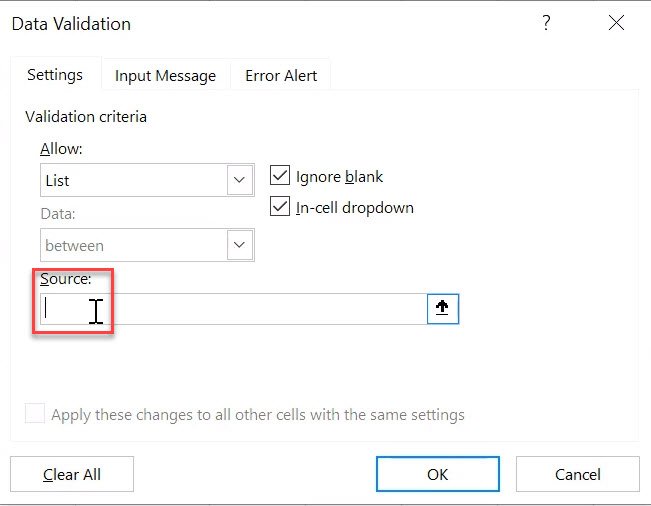
Click into the Source box. Make sure your insertion point is blinking in the Source box.

Now select over your list. Be sure to highlight every item you want included in the list.

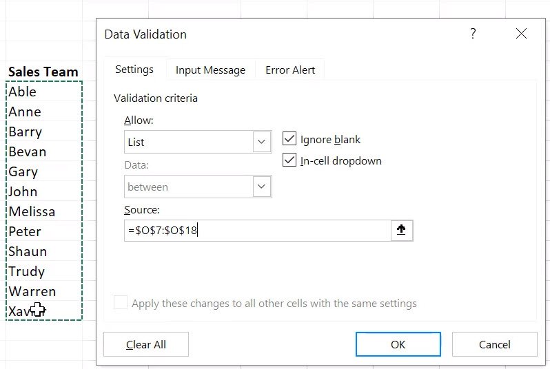
The range for the list should now be in the Source box. Click OK.

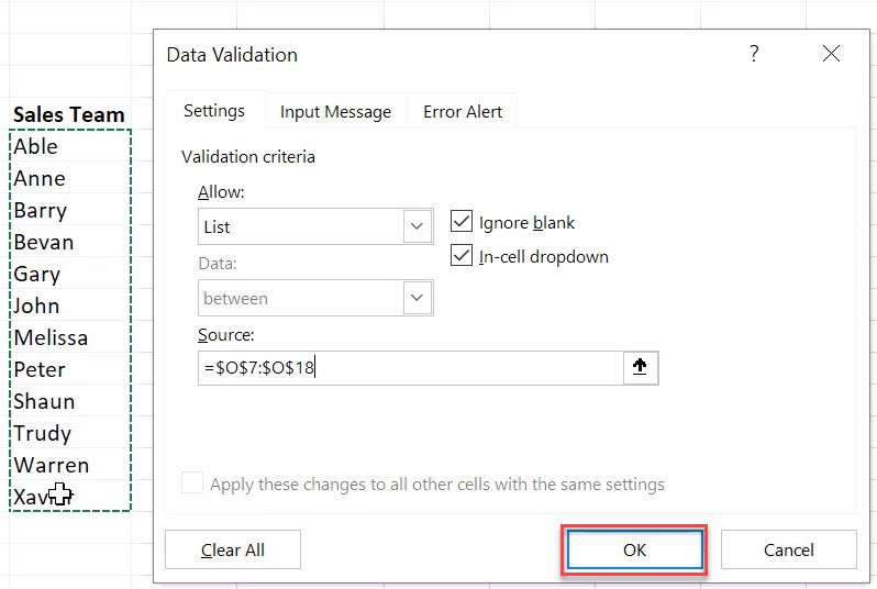
And your list should now be created.

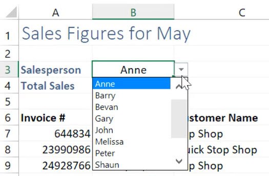
Note: this range is dynamic, which means if you update or change names on the original list, this will instantly update the drop-down list. For example, if we changed Anne’s name to Ann, this will be updated over in the drop-down list in cell B3.

The instruction above works for a drop-down list based on a list in the same worksheet, but what about a list from a different worksheet?

Option #2 – Create a Drop-Down List from a Different Worksheet

In this example, there are two worksheets. One is named ‘Drop down list’, which holds our Sales Figures and is where we want our drop-down list located. The other worksheet is called ‘Sales Team’. This worksheet has been created for the sole purpose of containing items that will be in our drop-down list. 

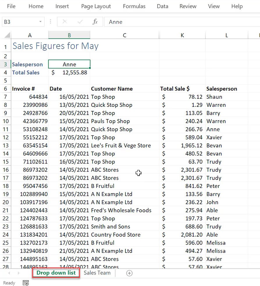
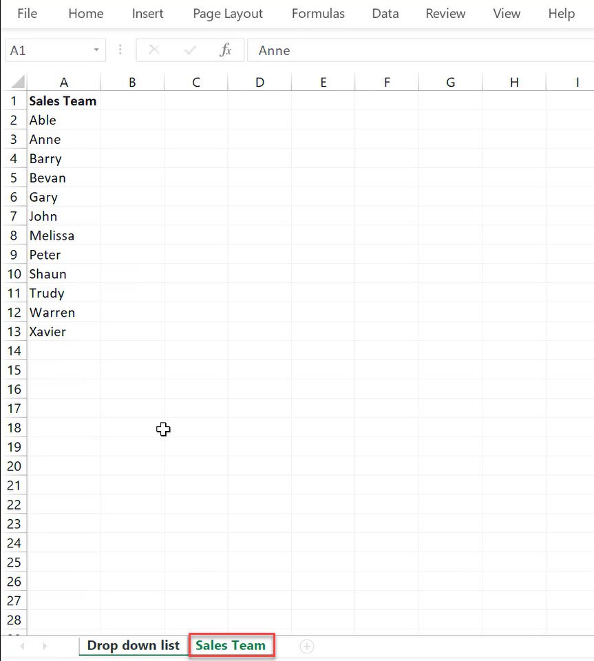
Select the cell you want the drop-down list on. For this example, we want the drop-down list on cell B3 on the Drop down list worksheet.

Select the Data tab and then Data Validation.

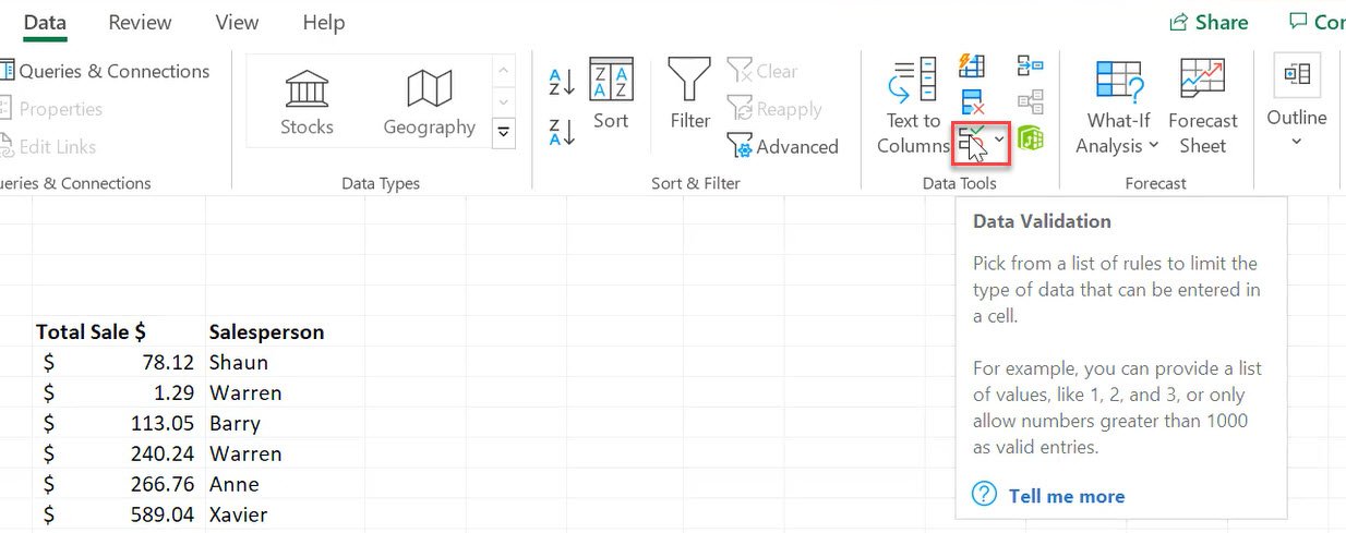
In settings, select List.

Click your insertion point into the Source text box.

Click onto the worksheet that holds the list. In this example, it is the Sales Team worksheet.

Note: if at this stage you are unable to click on to another worksheet, please refer to Option #3 below.

Highlight the list that you want as your drop-down list items.

The worksheet name, Sales Team, will now be included in the range in the Source box.

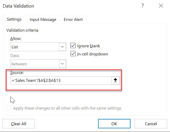
Click OK.

Your drop-down list should now be created in the Drop down list worksheet.

Tip: Sometimes it’s a good idea to hide the worksheet that contains the drop-down list items. This prevents others from tampering with the list items. To hide a worksheet, right-click the worksheet tab, and then select Hide.

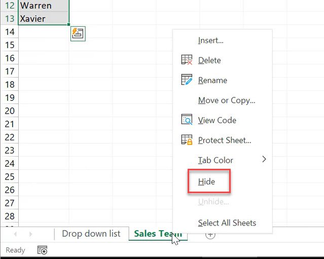
The worksheet will now be hidden. To edit the list at any time, just right-click any worksheet tab and select Unhide. Select the name of the hidden worksheet and then click OK..

Option #3 Create a Drop-Down List from a Different Worksheet (Older Versions Of Excel) 

If you are in an older version of Excel, in the Data Validation dialog box you cannot click into another worksheet when trying to source the list from another worksheet.

The following steps show you how to work around this.

Go to the worksheet that holds the drop-down list items. In this example that is the Sales Team worksheet.

Highlight your list.

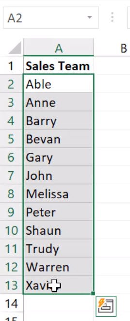
Click into the Name box, which is located on the very left of the Formula Bar.

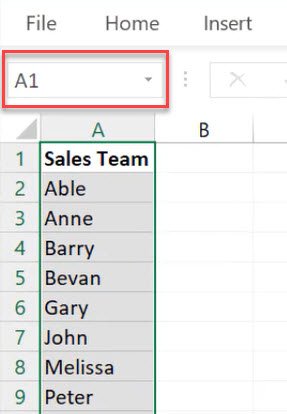
Delete the cell reference and type a name for the list.

Note: Do not put any spaces between the words. For this example, we will name the list SalesTeam.

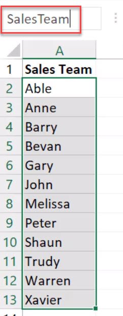
Press Enter and you have now given the list a name.

Return to the worksheet where you want your drop-down list. In this example, that is the Drop-down list worksheet.

Click on the cell where you are wanting the drop down list. Select the Data tab and then Data Validation.

Make sure you are in the Settings tab and select the drop-down arrow under Allow.

In Allow, select List.

Put your insertion point into the Source text box and type the named range you created, preceded by = (the equals sign), for example, =salesteam

Note: The list name is not case sensitive, you just need to be sure you spell it correctly.

Click OK.

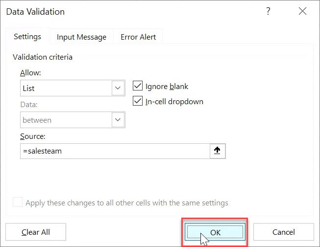
You should now have a drop-down list linked through to the named list items.

Watch the Excel how to create a drop-down list tutorial

[Watch on YouTube] / [Subscribe to our YouTube Channel]

Sharyn Baines, Trainer

Was this blog helpful? I’m here to empower your journey with Excel, aiming to make your daily tasks more efficient and boost your potential.

Share your thoughts in the Comments below – your insights not only enrich others, they also help me tailor future content to your needs.And if you’re looking to take a step further, join our exclusive ‘Insider Group‘. As a member, you’ll get early access to our latest tips, and in-depth tutorials. Sign up Today!”

Happy Excel-ling!!