Are you trying to count cells with text in Excel?
Are you wondering why the COUNT function in Excel returns a result of 0?
You’re not alone. Counting cells with text can be a bit of a struggle in Excel if you are unaware of which function to use when.
What's more, there are several different formula options available to help you quickly get the results you want.
In this blog I’ll explain why the COUNT function is returning a zero and I'll introduce you to 3 easy to use count functions and 9 super useful formula examples so that you can effortlessly count cells with text in Excel.
- Include text and values in a count
- Count only cells that contain text
- Count occurrences of specific text
- Count cells that don't contain specific text
- Count cells that contain partial matches of text
- Use the content of another cell to set the count criteria
- Count cells excluding formulas and cells containing spaces
- Count cells using multiple criteria
- Count cells using multiple criteria and wildcards
Why does the Count function in Excel return a result of 0?
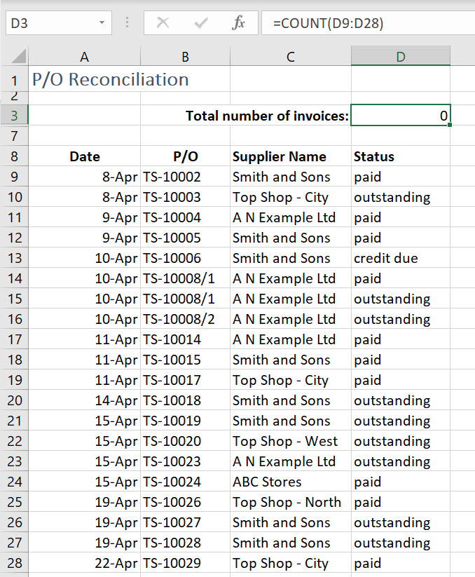
In the example below the COUNT function has been used to count the number of cells that contain text in the range D9 to D28. The formula is =COUNT(D9:D28).
Although there are 20 entries Excel returns the result as 0 (zero).
This is because the COUNT function is only looking for numbers. The cells below the Status column contain text. This is why the COUNT function returns a result of 0.
To count the entries in the range we need to use the COUNTA function.
Use the COUNTA function in Excel to count cells including text and values
With the simple addition of the letter ‘a’ after COUNT we can change the COUNT to the COUNTA function.
Using the count formula =COUNTA(D9:D28) Excel will count the number of cells that have any content, including text. We now have a result of 20, just what we were looking for. Please note, any cell with content will be counted, which means COUNTA will include errors and cells holding spaces, which means this could potentially give you an incorrect result.
I've included instruction on how to deal with this below.
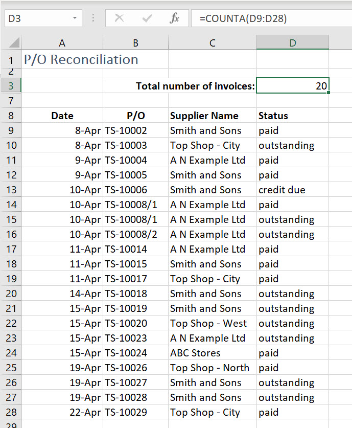
COUNTA function counts cells containing any type of information
The COUNTA function counts the number of cells that are not empty in a range.
I remember this function by saying to myself “count anything”.
It worked perfectly for us in our example above.
However, The COUNTA function counts cells containing any type of information, including error values and cells containing empty text ("").
Therefore, you can end up with a result that’s incorrect and be left wondering why Excel’s COUNTA function is not working.
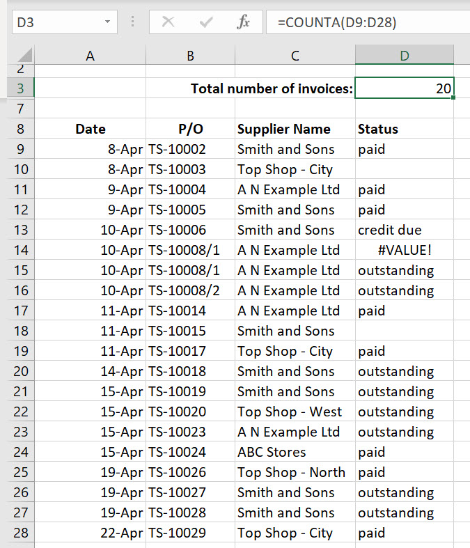
The COUNTA function example below shows cells D10 and D18 seeming to be empty and cell D14 holding an error #VALUE.
Still the function continues to return a count of 20 when we would prefer the empty cells and error #VALUE! to be excluded from the count.
Why is the COUNTA function not working?
The reason the COUNTA function is returning an incorrect result is because cells D10, D14 and D18 are included in the result.
Cell D14 holds an error and the COUNTA function includes errors in its result.
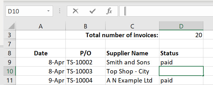
Cell D10 holds has a single space in it. The COUNTA function will see this as text and include it in the result.
Cell D18 holds a formula that is returning an empty cell (“”). Unfortunately, this is also seen to be text and included in the COUNTA function result.

Therefore, to get the correct results you may need to do a bit of data cleaning first.
Overcome COUNTA function problems
One way to overcome the COUNTA function counting all cells with content is to delete the content of any cells that contain errors, formulas or empty cells that contain spaces.
To do this I would recommend using Filter.
1. Select the range that contains the cells with spaces.
2. From the Data tab click Filter.
3. Click the filter drop-down arrow on the column that holds the empty cells.
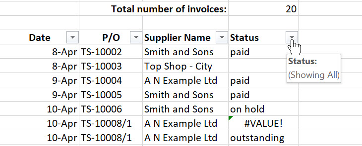
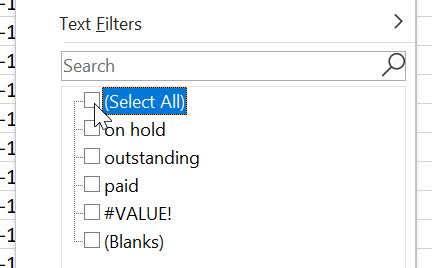
4. Remove the check from the Select All.
5. Now scroll to the bottom of the list and place a check next to any error you see, e.g. #VALUE!, and Blanks.
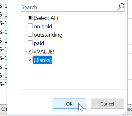
6. Click OK. Excel will now only display the rows that contain errors, formulas and spaces.
7. Select these cells.

8. Now press DELETE. The cells will now be empty and your COUNTA function will update and remove these cells from the result.

9. To turn Filtering off, from the Data tab click Filter again.
Using data cleaning method will help you use the COUNTA function with better results.
If you would prefer to keep the cells that are causing the COUNTA to be incorrect you will need to create a formula. Check the steps below for Excel COUNTA and COUNTIF to exclude formulas and cells containing a space.
Another way to overcome problems with using the COUNTA function is to be more specific about the text cells you are wanting to count.
This is where you can use COUNTIF or COUNTIFS for a more accurate result.
Excel count cells with only text
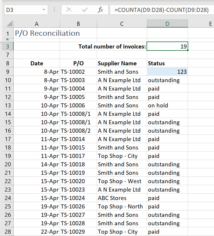
Using the COUNT and COUNTA function together in a formula we can easily find the number of cells that only contain text.
The count formula =COUNTA(D9:D28)-COUNT(D9:D28) shown in the example below is finding the number of cell with any content and then deducting the number of cells with numbers.
This then leaves you the number of cells that contain text only.
Note: you can also count cells with only text using the COUNTIF function and wildcards. To do this please see the notes below under Excel COUNTIF - count cells with only text.
Excel COUNTIF function – count occurrences of specific text
Excel’s COUNTIF function will count the number of cells that contain an exact match to specific text, for example, to count the number of purchase orders that still have a status of “outstanding”.
In the COUNTIF function example below you can see that the formula is =COUNTIF(D9:D28,"outstanding").
This asks Excel to look down the range D9 to D28 and only count the cells that contain the text outstanding.
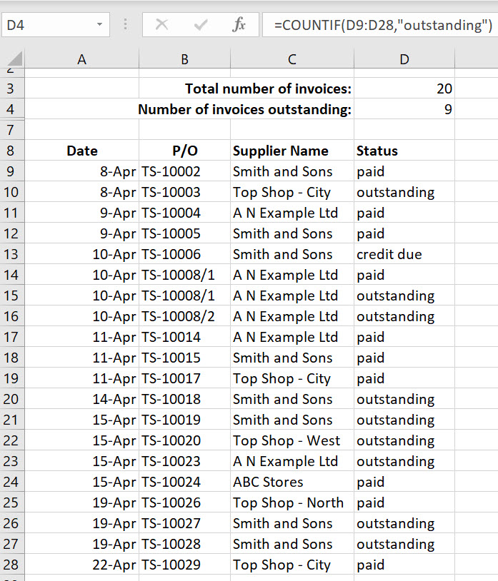
Note: the COUNTIF function has a limit of 255 characters and isn’t case-sensitive. OUTSTANDING, Outstanding, and outstanding will all work. However, you must make sure you place double quote marks around the text you specify so that Excel knows it is looking for text.
Excel COUNTIF function – count cells greater than, less than, equal to, not equal to
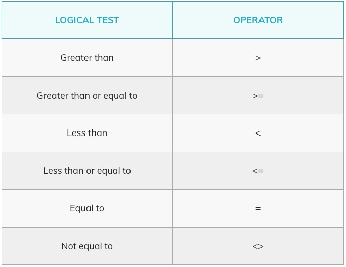
The COUNTIF function supports logical operators (>,<,<>,=).
In the example below, using the COUNTIF function and the Not equal operator we can count anything that isn’t ‘paid’.
This then allows us to include the purchase order that has a status of ‘on hold’. The formula is =COUNTIF(D9:D28,"<>paid")
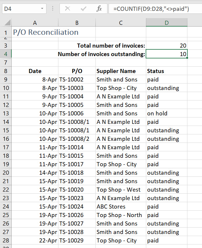
The following logical operators can be used within the criteria part of your formula. Just be sure to enclose the logical test within double quote marks, e.g., “<>paid”.
LOGICAL TEST | OPERATOR |
|---|---|
Greater than | > |
Greater than or equal to | >= |
Less than | < |
Less than or equal to | <= |
Equal to | = |
Not equal to | <> |
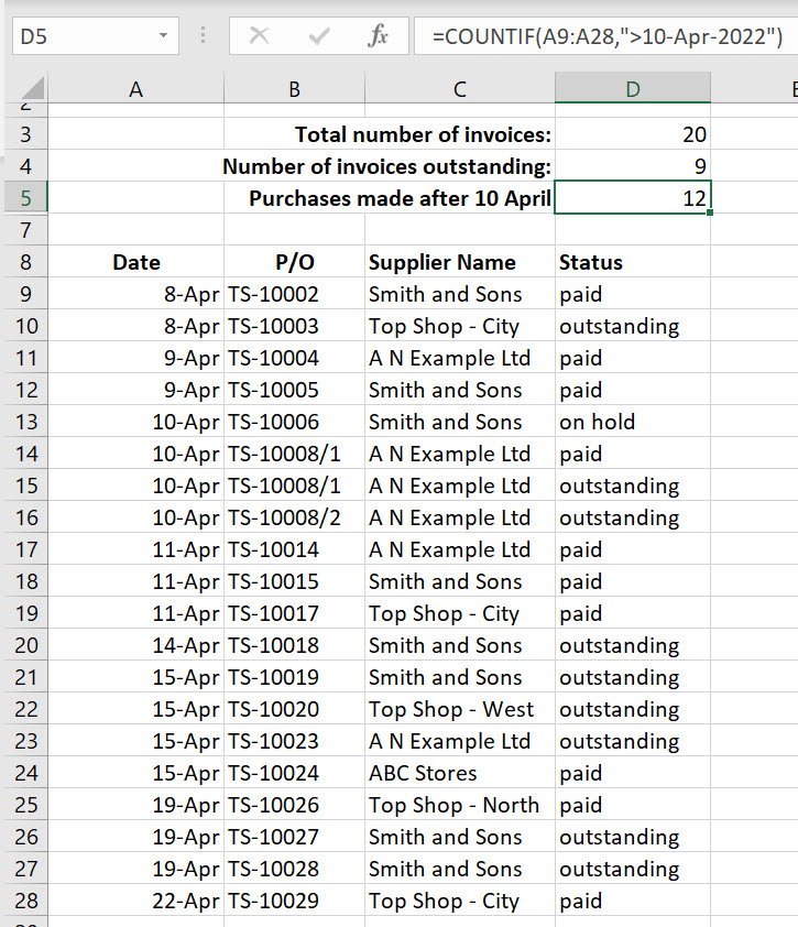
In the example below the COUNTIF function is counting how many cells contain a date greater than (after) the 10th of April 2022. The formula is =COUNTIF(A9:A28,">10-Apr-2022")
Excel COUNTIF function – count cells that have partial matches
The COUNTIF function supports wildcards for partial matching.
A wildcard is a symbol that substitutes an unknown character or set of characters.
The following wildcards can be used within the criteria part of your formula.
WILDCARD | OPERATOR | EXAMPLE |
|---|---|---|
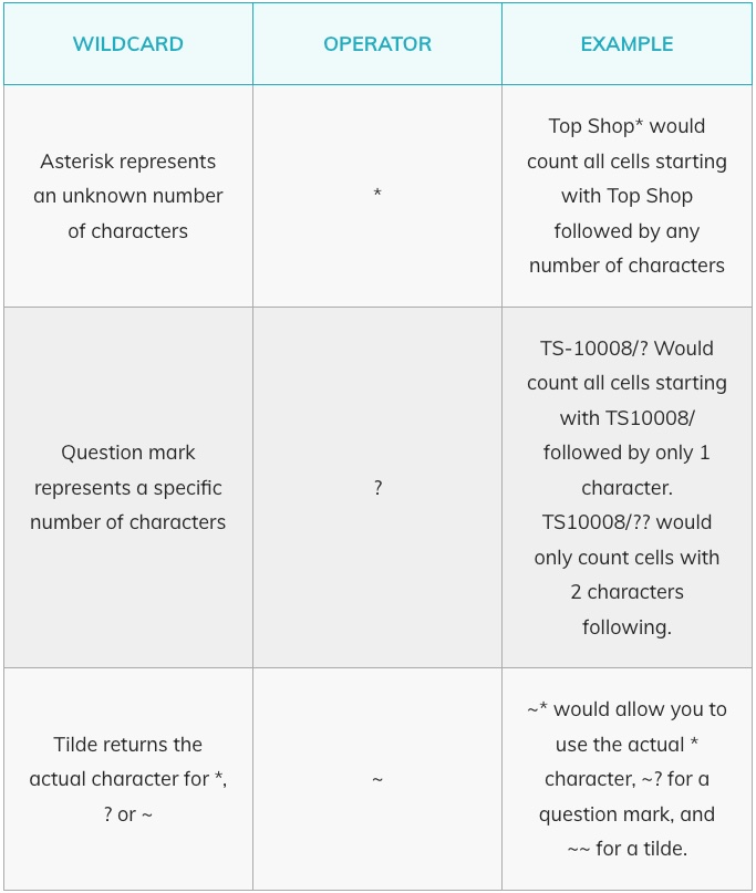
Asterisk represents an unknown number of characters | * | Top Shop* would count all cells starting with Top Shop followed by any number of characters |
Question mark represents a specific number of characters | ? | TS-10008/? Would count all cells starting with TS10008/ followed by only 1 character. TS10008/?? would only count cells with 2 characters following. |
Tilde returns the actual character for *, ? or ~ | ~ | ~* would allow you to use the actual * character, ~? for a question mark, and ~~ for a tilde. |
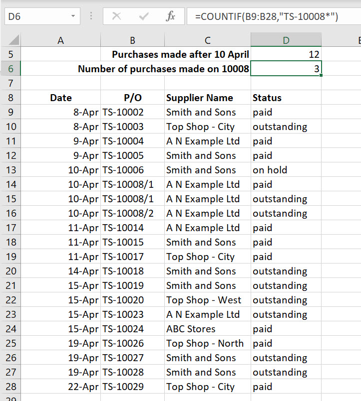
In the COUNTIF example below the formula =COUNTIF(B9:B28,"TS-10008*") is being used to count how many cells start with the purchase order number TS-10008.
The * at the end of the purchase order number states that any cells that start with the characters TS-10008 can be included, regardless of the number of characters that follow.
Therefore, the COUNTIF function will count cells B14, B15 and B16 even though they are listed as part 1 and part 2 of the TS-10008 purchase order number.
=COUNTIF(B9:B28,"TS-10008/?") would also work where the ? represents the single digit of the purchase order part number. However, if you had part numbers with 2 digits, e.g., TS-10008/12, this wouldn’t work.
Excel COUNTIF - count cells with only text
The COUNTIF function can be used to easily find cells that only contain text.
The count formula =COUNTIF(D9:D28,"*") is counting the number of cells that contain any kind of text, excluding cell D9 which holds a number.
Excel COUNTIF – use the content of another cell to set the count criteria
To reference a cell as part of your count criteria you need to string the operator to the cell reference.
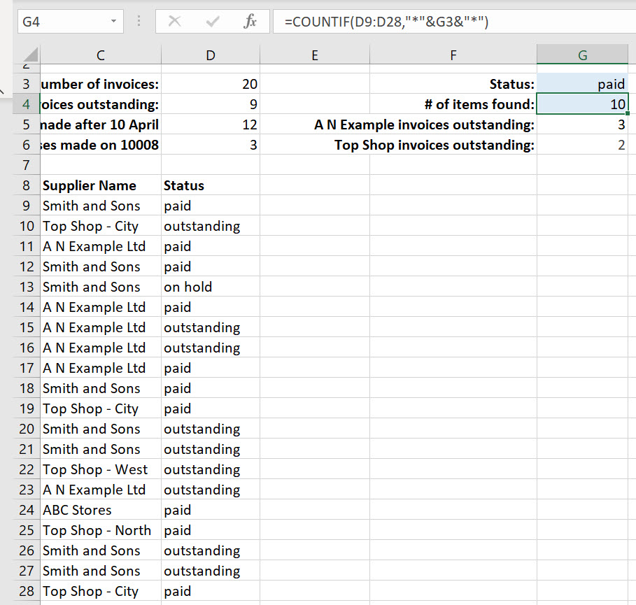
In the following COUNTIF example the formula =COUNTIF(D9:D28,"*"&G3&"*") is using the content of cell G3 to set the count criteria.
The trick here is enter the * and & symbols around the cell you want to reference. Be sure to follow the formula as shown in the example below.
Excel COUNTA and COUNTIF to exclude formulas and cells containing a space
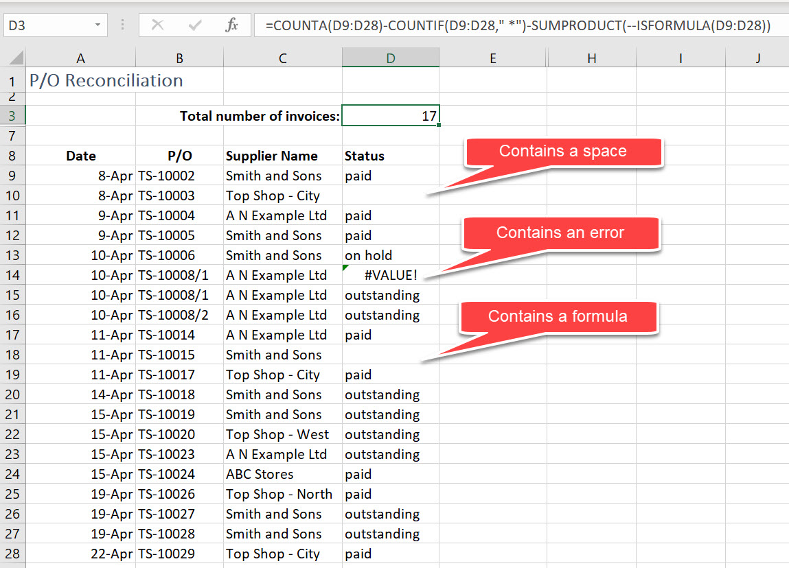
Using the COUNTA, COUNTIF and SUMPRODUCT functions together in a formula we can easily find the number of cells that only contain text, without having to delete the errors, formulas or cells containing spaces.
The formula is:
=COUNTA(D9:D28)-COUNTIF(D9:D28," *")-SUMPRODUCT(--ISFORMULA(D9:D28))
The COUNTA(D9:D28) is counting all cells that contain data within the range. This returns a result of 20.
The COUNTIF(D9:D28," *") includes a space and then an * inside double quote marks. This is counting all cells that start with a space regardless of the number of characters following. This returns a result of 1.
Note: This will allow you to count cells that contain any number of spaces. However, if there are leading spaces in front of cells that contain text you may need to clean these out first for this to work. For steps on how to do this see my blogs Remove spaces in Excel before and after text and Remove spaces Excel TRIM function misses.
SUMPRODUCT(--ISFORMULA(D9:D28) checks the range for any cells that contain a formula. The double negative signs change the result of TRUE or FALSE into 1s and 0s and the SUMPRODUCT returns the sum of these. This returns a result of 2.
Therefore, 20 minus 1 minus 2 = 17. The correct result.
Excel COUNTIFS function -set multiple criteria
COUNTIFS is like a COUNTIF but with the added power of counting cells that meet more than one (multiple) criteria.
The formula =COUNTIFS(C9:C28,"A N Example Ltd",D9:D28,"Outstanding") shown in the example below is used to count the number of outstanding purchase orders for the client A N Example Ltd.
Both criteria must be met for the cells to be counted.
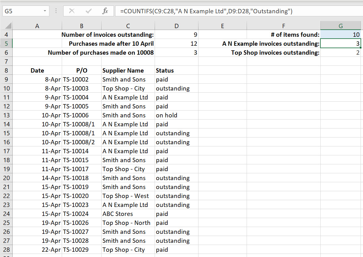
Note: it is important that the ranges you are evaluating are parallel to each other, i.e., in the example above the range for the first criteria is C9:C28. The range for the second criteria is D9:D28. Both ranges start and finish on the same row. Failure to do this will return an incorrect result.
Excel COUNTIFS function – use wildcards to count a partial match
The COUNTIF function supports wildcards (*,?) for partial matching.
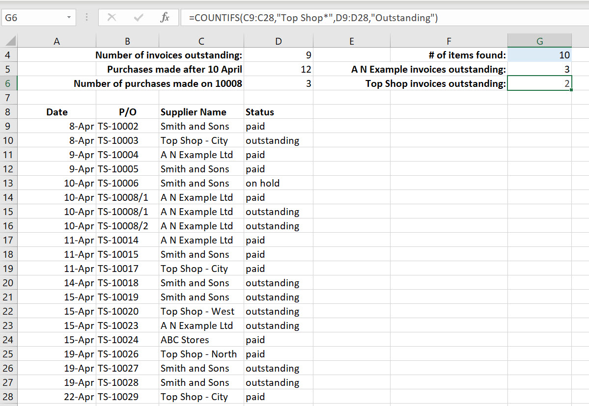
In formula example =COUNTIFS(C9:C28,"Top Shop*",D9:D28,"Outstanding") shown below is counting the number of cells that contain the text Top Shop and have a status of outstanding.
The * at the end of Top Shop is being used to specify that any cell that starts with the text Top Shop can be included, regardless of the characters that follow.
Therefore, the COUNTIFS function will count two cells that meet both criteria. Cells D10 and D22. D10 is the Top Shop – City branch and D22 is the Top Shop – West branch.
To Sum up
Using the COUNTA, COUNTIF and COUNTIFS functions, along with the formula examples I’ve covered, you should now have some great options to pop into your Excel toolkit.
I hope you found these super useful. Let me know in the Comments below.
If you enjoyed this post check out the related posts below.

