Have you ever tried to apply multiple filters to the same field in a Pivot Table, only to find that your first filter disappears as soon as you add the second one? It’s frustrating, right? Don’t worry—this blog is here to help! I’ll show you a quick, simple setting that will fix this issue and walk you through it step by step, complete with screenshots.
Excel Practice Files
Create an Excel Pivot Table
Let’s say you have a sales report where each record includes the name of an Account Manager, the client’s contact information, and the total sales value. You’ve been asked to create a report that shows only the clients managed by Anne and excludes any entries where the contact information is an email address or where the sales value is zero (0).
Creating a Pivot Table is the perfect way to build your report quickly.

The steps below explain how most people approach this task.
Create Excel Pivot Table Report
The first step is to create the Pivot Table report.
Tip: For clear instructions on how to do this, download the exercise file for this post and follow along with my video, which I have embedded in it.
Steps to Create a Pivot Table:
Step 1: Select Your Data: Highlight the entire dataset, including the headers. Note: If your data is formatted as a table, you don’t need to select it. Jump straight to step 2.

Step 3: Set Up Your Pivot Table Fields:
- Drag Contact Info into the Rows area.
- Drag Account Mgr into the Columns area.
- Drag Value into the Values area (Excel will automatically sum this field).

Step 4: (Optional) Apply Basic Formatting:
- Format the values as currency or number, depending on your dataset.
- Rename the Pivot Table fields if needed for clarity.
Apply Filters to Excel Pivot Table
With your Pivot Table now set up and organised, it’s time to refine the data to meet the specific requirements of your report.
In this case, we need to filter the data to show only the clients managed by Anne, exclude any rows where the contact information is an email address, and ensure no records with a sales value of zero are included.
This is where filtering plays a crucial role—and where the default Pivot Table settings might cause unexpected issues.
Let’s dive into the filtering process.
Step 1: Begin by filtering the Account Manager field to hide all records where Steve is the Account Manager. [1] Click on the dropdown arrow in the Account Manager column, [2] uncheck “Steve,” and click OK.

Step 2: Next, you want to exclude all email addresses from the Contact field. To do so, [1] click on the dropdown arrow in the Contact column, [2] type “@” in the search box, [3] uncheck “Select All,” and then [4] select “Add current selection to filter” before clicking OK.

Step 3: Now, we will filter the Contact field again, this time for values greater than zero (0). [1] Click the dropdown arrow in the Contact column, [2] click “Value Filters”, [3] click “Greater Than”. [4] Type 0 in the Value Filter box and then click OK.


Result: After applying the second filter to the Contacts field, the records are no longer filtered properly. All of the contact email addresses reappear! The filter on the Contact field overwrote the previous filter, and you’re back to square one.

The Problem: The default setting in Excel only allows one filter per field in a Pivot Table. So, every time you add a new filter, it replaces the previous one. It’s like Excel doesn’t understand what you’re trying to do, and it’s incredibly frustrating.
Relatable? Let’s fix it!
How to Apply Multiple Filters to the Same Field in an Excel Pivot Table
Good news! There’s an easy fix. Just follow these steps:
Step 1: Click anywhere inside your Pivot Table.
Step 2: Go to the Pivot Table Analyze tab (or right-click any cell inside the pivot table) and select Pivot Table Options.

Step 3. In the dialog box, [1] go to the Totals & Filters tab. [2] Check the box for Allow Multiple Filters per Field.
Step 4: Click OK.

Note: You don’t need to enable this feature for every Pivot Table in your workbook; once activated, it remains active for all future Pivot Tables within the same workbook. However, you’ll need to enable this setting for each individual file you work with.
Filter the Pivot Table with ‘Allow multiple filters per field’ Enabled
Once you have enabled “Allow multiple filters per field’, test the new setting by repeating the steps:
- Remove all records for “Steve” from the Account Mgr field.
- Remove all email addresses from the Contact field.
- Remove all records where the Value is zero (0).
- Both filters now work together seamlessly on the same field. When we check the filter settings, we see that both the Value Filter and the Label Filter are active.

It’s so satisfying to see Excel finally behaving the way you want it to!

Pivot Table Pro Tips
Take your Pivot Table to the next level with these tips:
- In our example, we now see Anne’s data is replicated in the ‘Grand Total’ column. To remove Grand Totals, right-click the ‘Grand Totals’ heading, and then select Remove Grand Total for a cleaner look, eliminating repetitive columns and allowing you to focus on the important data.

- Practice using the Search Box to Quickly find specific data by typing keywords into the filter search box.

These small changes can save you heaps of time and make your data easier to work with.
Conclusion: Allow Multiple Filters per Pivot Table Field
And there you have it! With just one small setting change, you can apply multiple filters to the same field in your Pivot Table. No more frustration, just efficient data analysis.
Was this guide helpful? Let me know in the comments below! For more Excel tips and tricks, check out my other tutorials or sign up for my online courses.
Share the Knowledge: Know someone who struggles with Pivot Tables? Share this blog with them!
Watch The Excel Video Tutorial
[Watch on YouTube] / [Subscribe to our YouTube Channel]
Excel Practice File Download
Want to Learn Excel Properly?
Join the Excel at Work Learning Hub
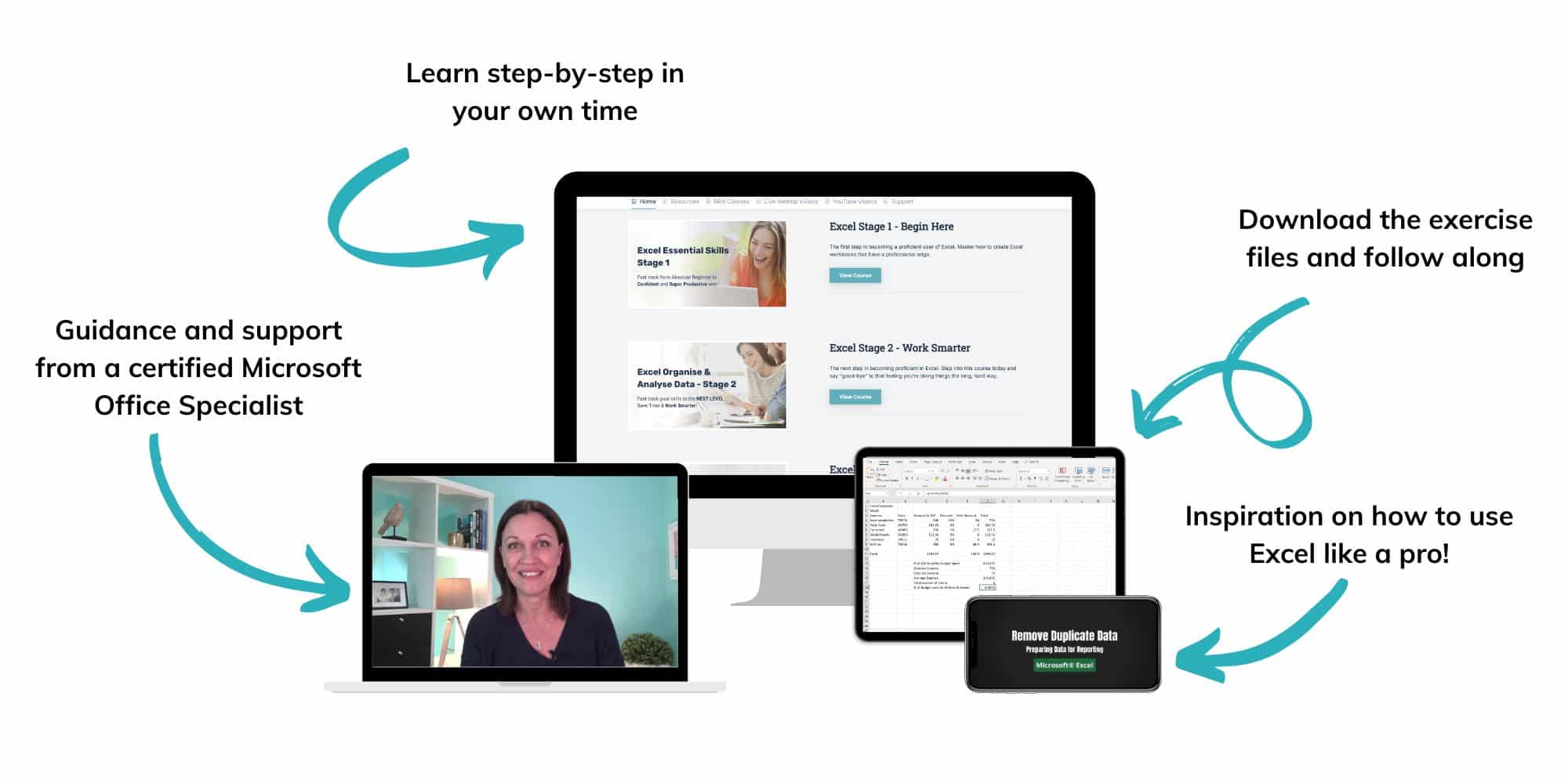
The Excel at Work Learning Hub is an online self-paced Excel training membership designed for people who use Excel at work—in offices, on sites, in schools, in small businesses, and everywhere in between.
Go from Beginner to Confident – Guaranteed!
Only $59NZ /month
Cancel anytime • No pressure • 14-day 100% Money Back Guarantee

Certified Microsoft Office Specialist
Was this blog helpful? I’m here to empower your journey with Excel, aiming to make your daily tasks more efficient and boost your potential.
Share your thoughts in the Comments below – your insights not only enrich others, they also help me tailor future content to your needs.
And if you’re looking to take a step further, join our exclusive ‘Insider Group‘. As a member, you’ll receive Weekly Super-Tips, and early access to in-depth tutorials. Sign up Today!
Happy Excel-ling!!