Excel – How do I move the negative sign in front of the number?

Anyone that regularly imports data into Excel will be familiar with the process of “data cleaning”. This is where you need to remove spaces and irrelevant data in order to get the data fit for use in Excel.

I recently had an excellent question regarding working with data imported into Excel where negative numbers are imported with the negative sign to the right of the number, e.g. 500-. These numbers are commonly referred to as “mirrored negatives”.

This is a common data cleaning challenge (and a real “pain in the tech”). The mirrored negative problem isn’t just an aesthetic one. Sadly Excel doesn’t recognise these numbers as negatives, which adds another layer of frustration to the entire importing process.

So how do you move the negative sign in front of the number?

Well it’s not a one step process. But bear with me. I’ll break down the process so that it’s easy to identify each part.

First you need to identify if the cell contains a mirror negative. Using the IF and RIGHT functions we can easily identify this. In the screen shot below I have used the formula in F4 to see if the last character in cell E4 is a negative sign. If it is TRUE is returned. If it isn’t FALSE is returned.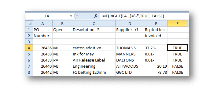

Using this formula we can identify if the cell holds a negative. But we want to do more than just identify the problem. We want to move the pesky negative sign. To do this it would make sense to substitute the TRUE part of the IF function with a formula that will move the sign.

Cell F4 in the screen below shows a formula using the LEFT and LEN functions. Let me break the formula down for you.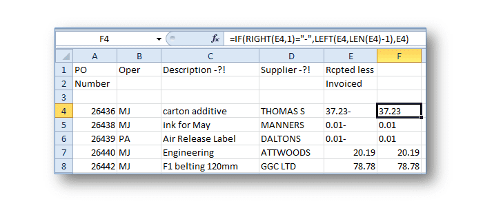

The LEFT function returns the first characters of the content held in cell E4.

The LEN function specifies how many characters are held in E4.

Putting the two functions together means you can easily pull the characters you require from the cell. In the example above the LEN function calculates that 6 characters are held in cell E4.

Putting this together with the LEFT function and adding minus 1 to the formula pulls only 5 of the first 6 characters of the cell leaving the negative sign behind.

We now have the number without the negative sign. Inserting *-1 into the formula multiplies the number by negative 1 therefore placing the negative sign in front of it.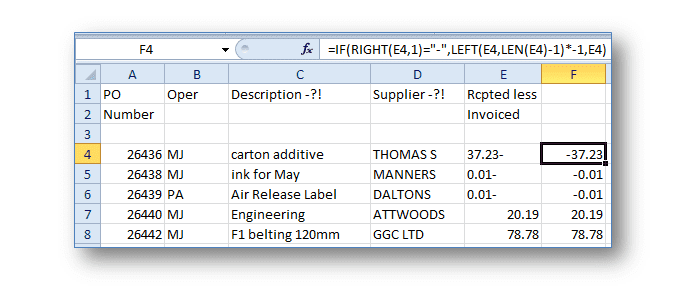

The last part of the IF function ensures any cell that doesn’t hold a mirrored negative is returned as is.

Note: you may have one more problem to overcome. If the number returned in F4 is still seen to be text inserting the VALUE function into the formula ensures the number is always returned as a value, not text.
=IF(RIGHT(E4,1)=”-“,VALUE(LEFT(E4,LEN(E4-1)*-1,E4)

The very last step in the process is to copy the formula into cells F5 to F8. Using Copy, Paste Special, Values the formula can then be turned back into a format suitable for use.